A first quantum simulation — a free Gaussian wave packet on a ring

Marcin Płodzień — Institute of Theoretical Physics, Jagiellonian University in Kraków
ORCID 0000-0002-0835-1644 · github.com/MarcinPlodzien · www

Quantum Many-Body Simulation — Chapter 1 — Computational toolbox

1. Introduction

This notebook uses a computer as a laboratory: a quantum system is set up, evolved in time, measured, and compared with what pencil and paper predict.

1.1 Theory, numerics, experiment

Physics has three legs. Theory produces equations and, in the lucky cases, closed-form solutions. Experiment produces numbers with error bars. Numerics sits in between: it takes the equations seriously, solves them on a computer for systems that are far too complicated for pencil and paper, and produces numbers that can be compared with both. Almost everything we know quantitatively about interacting quantum matter — superconductors, cold atoms in optical lattices, the noise in a real quantum processor — comes from that third leg.

A numerical simulation always follows the same four steps:

1. A continuous equation. Here: the Schrödinger equation, an equation for a function \(\psi(x,t)\) of a continuous variable \(x\) — infinitely many numbers.
2. Discretisation. We replace the continuum by a finite set of numbers: the values of \(\psi\) at \(N_x\) selected points \(x_0, x_1, \ldots, x_{N_x-1}\). A computer can hold those. Derivatives, integrals and the equation itself must be re-expressed in terms of this finite list.
3. An algorithm. A recipe that turns the list at time \(t\) into the list at time \(t + \Delta t\) — a finite number of additions and multiplications.
4. A result with a controllable error. This is the part beginners forget. The output is never the exact answer. It differs from it by a discretisation error (we used \(N_x\) points instead of infinitely many) and by a round-off error (the computer stores each number with about \(16\) decimal digits). A simulation is only worth something if you can show that these errors are small and that you know how to make them smaller.

1.2 Why our first system has a known exact solution

One rule of computational physics comes before all others:

Numerical practice. Never trust a simulation you have not tested against something you know independently. The first run of any new code is on a problem whose answer you already have — an exact solution, a conservation law, a known limit, or a second, completely different algorithm.

A program with a wrong sign, a factor of \(2\), or an index off by one will happily run and produce smooth, plausible, beautifully coloured, wrong pictures. Nothing in the output says “I am wrong”. The only defence is a reference.

The free particle — no forces, no potential — is a natural first test case. Its Schrödinger equation can be solved in closed form for a Gaussian initial state, giving formulas for the position, the width, and the full wave function at any time. So we can put the exact curve and the computed curve on the same plot and measure the distance between them.

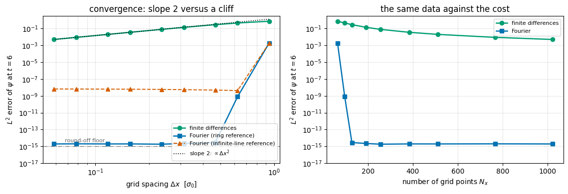
“Agreement” has a precise meaning, stronger than “the curves look the same”: the difference shrinks, when we refine the grid, in the way the theory of the method predicts — for the finite-difference method we will derive, the error must fall like \((\Delta x)^2\); halve the grid spacing and the error must drop by a factor of four. If it does, the code is almost certainly right. If it does not, something is broken, even when the pictures look fine.

1.3 The physics: a spreading wave packet

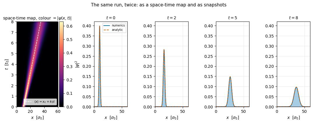
The system itself is the “hello world” of quantum dynamics. A particle is prepared in a Gaussian wave packet: a lump of probability of width \(\sigma_0\), centred at \(x_c\), carrying an average momentum \(\hbar k_0\). It is the closest a quantum particle gets to a classical particle with a definite position and velocity. Then we let go. Two things happen at once:

• the lump moves with the group velocity \(\hbar k_0/m\), exactly as a classical particle would;
• the lump spreads, because a localised state necessarily contains a range of momenta (\(\sigma_x \sigma_k \ge 1/2\) — the uncertainty relation), and different momentum components travel at different speeds. A classical swarm of particles with the same spread of velocities spreads in exactly the same way (Section 8.3); the quantum part is that a localised state cannot avoid having that spread.

The same spreading happens

• to an electron emitted from a tip or a photocathode, and in every simulation of electron transport;
• to a cloud of ultracold atoms the instant the trap holding it is switched off — the standard “time-of-flight” measurement in every cold-atom laboratory reads the momentum distribution off the expansion of the cloud;
• in matter-wave interferometry, where a single atom or molecule is split into two packets that spread, travel, and are recombined to interfere.

The time scales differ enormously (Section 2 computes them): a \(1\,\mathrm{nm}\) electron packet doubles its width in a few tens of femtoseconds, while a \(1\,\mu\mathrm{m}\) cloud of rubidium atoms takes a few milliseconds — eleven orders of magnitude apart, and yet, as we will see, the same simulation describes both.

1.4 Road map

• Section 2 — the free Schrödinger equation in SI units, and non-dimensionalisation: how we strip \(\hbar\) and \(m\) out of the equation by measuring lengths, times and energies in units built from the problem itself.
• Section 3 — the exact solution of the free Schrödinger equation: Fourier transform, Gaussian integral, free propagation, transform back. Results: \(\langle x \rangle(t)\), \(\sigma(t)\), the chirp, the uncertainty product.
• Section 4 — the grid: what an array holds, what periodic boundary conditions mean, which wave numbers a grid can represent, and what happens when you ask for one it cannot (aliasing).
• Section 5 — first contact with the numbers: build the packet, check its norm, mean position and width with sums instead of integrals.
• Section 6 — method A, finite differences: Taylor expansion, the three-point Laplacian, the circulant Hamiltonian, its exact eigenvalues, and the numerical dispersion relation — the reason a finite-difference packet moves slightly too slowly.
• Section 7 — method B, the Fourier (spectral) method: with periodic boundaries the kinetic energy is diagonal in Fourier space, so one FFT, one multiplication and one inverse FFT give the exact answer.
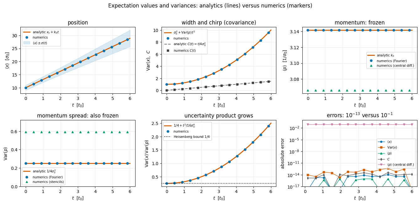
• Section 8 — expectation values and variances, analytics and numerics side by side: Ehrenfest’s theorem, \(\langle x\rangle\), \(\langle p\rangle\), \(\mathrm{Var}(x)\), \(\mathrm{Var}(p)\), the covariance, the uncertainty product — and two different ways of computing momenta on a grid.
• Section 9 — the numerics-versus-analytics verdict: convergence plots, conservation laws, cost.
• Section 10 — animations: a reusable function that turns a stack of snapshots into an animated GIF embedded in the notebook.
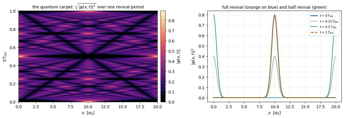
• Section 11 — what the ring does to us: wrap-around, self-interference, the image sum, and exact revivals.
• Section 12 — summary, a reusable workflow checklist, exercises and references.

What you will learn

Physics

• the free Gaussian wave packet: group velocity, spreading law \(\sigma(t) = \sigma_0\sqrt{1 + (t/2\sigma_0^2)^2}\), the position-dependent “chirp”, phase velocity versus group velocity, the growth of the uncertainty product;
• why a momentum distribution never changes for a free particle;
• Ehrenfest’s theorem (\(d\langle x\rangle/dt = \langle p\rangle\)), the ballistic variance law \(\mathrm{Var}(x)(t) = \mathrm{Var}(x)(0) + \mathrm{Var}(p)\,t^2\) and the position-momentum covariance;
• what periodic boundary conditions do: self-interference and exact quantum revivals on a ring.

Numerical methods

• non-dimensionalisation; grids, discretisation error, round-off error, machine precision;
• the three-point Laplacian and its \(O(\Delta x^2)\) error; circulant matrices and their plane-wave eigenvectors;
• numerical dispersion; the sampling theorem and aliasing;
• the Fourier (spectral) method, fft/ifft/fftfreq, spectral accuracy, \(O(N\log N)\) cost;
• how to run and read a convergence test (log-log plot, fitted slope).

Implementation practice

• turning integrals into array sums, and formulas into vectorised code;
• jax.jit, jax.vmap and lax.scan in their simplest possible setting;
• validating every step with assert against the analytic result;
• producing animated GIFs from matplotlib and embedding them in a notebook without leaving files behind.

Configuration

Every notebook of this course starts with the same cell. Choose where to run (DEVICE) and the floating-point precision (PRECISION): "double" = float64/complex128 (default, recommended for physics), "single" = float32/complex64 (half the memory, faster on consumer GPUs, but watch the round-off). All code below derives its dtypes from RDTYPE/CDTYPE and its check tolerances from TOL, so nothing else needs to change.

Code

# ==============================================================================
# CONFIGURATION  -- adapt to your hardware, then run the notebook top to bottom
# ==============================================================================
DEVICE    = "auto"     # "auto": use a GPU if JAX finds one, else CPU | "cpu" | "gpu"
PRECISION = "double"   # "double": float64/complex128 | "single": float32/complex64

import os
if DEVICE == "cpu":
    os.environ["JAX_PLATFORMS"] = "cpu"          # must be set BEFORE jax is imported

import string
from functools import partial

import math
import numpy as np
import jax
import jax.numpy as jnp
from jax import lax

# Precision is configurable: "double" = float64/complex128 (default; needed for long time evolutions and
# tight validation), "single" = float32/complex64 (half the memory, faster on consumer GPUs).
jax.config.update("jax_enable_x64", PRECISION == "double")
RDTYPE = jnp.float64 if PRECISION == "double" else jnp.float32       # real dtype
CDTYPE = jnp.complex128 if PRECISION == "double" else jnp.complex64  # complex dtype of all states/operators
TOL = 1e-10 if PRECISION == "double" else 1e-4                       # tolerance for sanity checks (asserts)
_LETTERS = string.ascii_letters  # the 52 einsum index labels a-z, A-Z

import time
import matplotlib.pyplot as plt

if DEVICE == "gpu" and jax.default_backend() == "cpu":
    print("WARNING: DEVICE='gpu' requested but JAX found no GPU -- running on CPU.")
print(f"JAX {jax.__version__} | backend: {jax.default_backend()} | devices: {jax.devices()}")
print(f"precision: {PRECISION} -> real {RDTYPE.__name__}, complex {CDTYPE.__name__}, check tolerance TOL={TOL:g}")

JAX 0.11.0 | backend: cpu | devices: [CpuDevice(id=0)]
precision: double -> real float64, complex complex128, check tolerance TOL=1e-10

2. The equation, and how to get rid of \(\hbar\) and \(m\)

2.1 The free Schrödinger equation in SI units

A particle of mass \(m\) moving in one dimension with no forces acting on it is described by a wave function \(\Psi(X,T)\) obeying the time-dependent Schrödinger equation, introduced in [1],

\[ i\hbar \frac{\partial \Psi(X,T)}{\partial T} \;=\; -\frac{\hbar^2}{2m}\frac{\partial^2 \Psi(X,T)}{\partial X^2} . \tag{1} \]

Capital \(X\) and \(T\) are a position in metres and a time in seconds. The right-hand side is the kinetic-energy operator \(\hat p^2/2m\) with \(\hat p = -i\hbar\,\partial_X\); there is no potential term, which is exactly what “free” means. The physical content of \(\Psi\) is the Born rule, introduced in [2]: \(\vert\Psi(X,T)\vert^2\,dX\) is the probability of finding the particle in \([X, X+dX]\), and

\[ \int_{-\infty}^{\infty} \vert\Psi(X,T)\vert^2 \, dX = 1 \qquad \text{for all } T . \]

2.2 Why we never type \(\hbar\) into a computer

In SI units \(\hbar \approx 1.05\times10^{-34}\,\mathrm{J\,s}\) and an electron mass is \(\approx 9.1\times10^{-31}\,\mathrm{kg}\). If we fed those numbers to a computer, every intermediate quantity would be a tiny or a huge number, we could not tell a “small” error from a “large” one, and — worse — the result would be specific to one particle. The cure is non-dimensionalisation: measure every quantity in units built out of the problem itself, so that the equation contains only pure numbers.

The free particle has one peculiarity. Equation (1) contains two constants, \(\hbar\) and \(m\). From them alone you cannot build a length: \(\hbar\) has units \(\mathrm{J\,s} = \mathrm{kg\,m^2\,s^{-1}}\) and \(m\) has units \(\mathrm{kg}\), so \(\hbar/m\) has units \(\mathrm{m^2\,s^{-1}}\) — a diffusion constant, not a length. The free particle has no intrinsic length scale. (A harmonic trap of frequency \(\omega\) would supply one, \(\sqrt{\hbar/m\omega}\).)

So we choose one. The only length in the problem is the one we put into the initial state: the initial width \(\sigma_0\) of the packet. Define

\[ x_0 \equiv \sigma_0 \qquad (\text{unit of length}). \]

2.3 Substituting the scaled variables

Write the position and the time as (a pure number) \(\times\) (a unit):

\[ X = x_0\, x , \qquad T = t_0\, t , \]

where \(x\) and \(t\) are dimensionless and \(t_0\) is a unit of time still to be chosen. By the chain rule,

\[ \frac{\partial}{\partial T} = \frac{1}{t_0}\frac{\partial}{\partial t}, \qquad \frac{\partial^2}{\partial X^2} = \frac{1}{x_0^2}\frac{\partial^2}{\partial x^2} . \]

The wave function must be rescaled too, because it is not dimensionless: \(\vert\Psi\vert^2\) is a probability density, so \(\Psi\) has units \(\mathrm{m}^{-1/2}\). Define

\[ \psi(x,t) \;\equiv\; \sqrt{x_0}\; \Psi(x_0 x,\; t_0 t) . \]

The factor \(\sqrt{x_0}\) is exactly what is needed to preserve the normalisation:

\[ \int \vert\Psi\vert^2\, dX \;=\; \int \frac{\vert\psi\vert^2}{x_0}\; x_0\, dx \;=\; \int \vert\psi\vert^2\, dx \;=\; 1 . \]

Substituting into Eq. (1) and cancelling the common factor \(x_0^{-1/2}\):

\[ \frac{i\hbar}{t_0}\,\frac{\partial \psi}{\partial t} \;=\; -\frac{\hbar^2}{2m x_0^2}\,\frac{\partial^2 \psi}{\partial x^2} . \]

Now divide both sides by the energy unit \(E_0 \equiv \hbar/t_0\):

\[ i\,\frac{\partial \psi}{\partial t} \;=\; -\frac{\hbar\, t_0}{2m x_0^{2}}\,\frac{\partial^2 \psi}{\partial x^2} . \]

The factor in front of the derivative, \(\hbar t_0/(m x_0^2)\), is a pure number — check the units: \(\mathrm{J\,s}\cdot\mathrm{s}/(\mathrm{kg}\,\mathrm{m^2}) = 1\) — and \(t_0\) is still ours to choose. Choose it so that the whole coefficient is exactly \(1/2\):

\[ \frac{\hbar\, t_0}{m x_0^{2}} = 1 \qquad \Longrightarrow \qquad \boxed{\; t_0 = \frac{m x_0^{2}}{\hbar} \;} \]

and the equation becomes, once and for all,

\[ i\,\frac{\partial \psi(x,t)}{\partial t} \;=\; -\frac{1}{2}\,\frac{\partial^2 \psi(x,t)}{\partial x^2} . \tag{2} \]

No \(\hbar\), no \(m\). This is the equation we will solve for the rest of the notebook. It is what the common phrase “units with \(\hbar = m = 1\)” stands for.

2.4 The full set of units

Everything else follows from \(x_0\) and \(t_0 = m x_0^2/\hbar\):

quantity	unit	in terms of \(x_0\)
length	\(x_0 = \sigma_0\)	chosen
time	\(t_0 = m x_0^2/\hbar\)	derived
energy	\(E_0 = \hbar/t_0 = \hbar^2/(m x_0^2)\)	derived
wave number	\(k_{\rm unit} = 1/x_0\)	reciprocal length
momentum	\(p_0 = \hbar/x_0\)	since \(p = \hbar k\)
velocity	\(v_0 = x_0/t_0 = \hbar/(m x_0)\)	derived

To go back to the real world you multiply by the unit. A dimensionless time \(t = 3\) means \(T = 3\, m x_0^2/\hbar\) seconds; a dimensionless wave number \(k = 2\) means a real momentum \(2\hbar/x_0\). Let us put numbers on that for our two physical examples.

Code

# ==============================================================================
# STEP 0: the unit system, for two real experiments
#   We choose x_0 = sigma_0 (the initial width of the packet).  Everything else
#   follows:  t_0 = m x_0^2 / hbar,  E_0 = hbar / t_0,  v_0 = x_0 / t_0.
#   This cell is pure bookkeeping -- no quantum mechanics happens here.
# ==============================================================================
HBAR_SI = 1.054571817e-34        # reduced Planck constant           [J s]
M_ELECTRON = 9.1093837015e-31    # electron mass                     [kg]
AMU = 1.66053906660e-27          # atomic mass unit                  [kg]
M_RB87 = 87.0 * AMU              # mass of a rubidium-87 atom        [kg]
EV = 1.602176634e-19             # one electronvolt                  [J]


def unit_system(mass_kg, x0_m):
    """Units of the non-dimensional free Schrodinger equation, for a given mass and length unit.

    MATH
        t_0 = m x_0^2 / hbar      (unit of time)
        E_0 = hbar / t_0 = hbar^2 / (m x_0^2)   (unit of energy)
        v_0 = x_0 / t_0 = hbar / (m x_0)        (unit of velocity)
    Returns a dict of floats in SI units.
    """
    t0 = mass_kg * x0_m**2 / HBAR_SI
    return {"x0_m": x0_m, "t0_s": t0, "E0_J": HBAR_SI / t0, "v0_mps": x0_m / t0}


cases = [("electron,  x_0 = 1 nm     ", M_ELECTRON, 1e-9),
         ("Rb-87 atom, x_0 = 1 micron", M_RB87, 1e-6)]

print(f"{'system':28s} {'t_0 [s]':>12s} {'E_0 [J]':>12s} {'E_0 [eV]':>12s} {'E_0/h [Hz]':>12s} {'v_0 [m/s]':>12s}")
for name, mass, x0 in cases:
    u = unit_system(mass, x0)
    print(f"{name:28s} {u['t0_s']:12.3e} {u['E0_J']:12.3e} {u['E0_J']/EV:12.3e} "
          f"{u['E0_J']/(2*np.pi*HBAR_SI):12.3e} {u['v0_mps']:12.3e}")

# The spreading time (derived in Section 3): the packet's width has grown by sqrt(2)
# after t = 2 sigma_0^2 in our units, i.e. after T_spread = 2 m sigma_0^2 / hbar in seconds.
print()
for name, mass, x0 in cases:
    t_spread = 2.0 * mass * x0**2 / HBAR_SI
    print(f"{name:28s} spreading time T_s = 2 m sigma_0^2/hbar = {t_spread:10.3e} s")

system                            t_0 [s]      E_0 [J]     E_0 [eV]   E_0/h [Hz]    v_0 [m/s]
electron,  x_0 = 1 nm           8.638e-15    1.221e-20    7.620e-02    1.842e+13    1.158e+05
Rb-87 atom, x_0 = 1 micron      1.370e-03    7.698e-32    4.805e-13    1.162e+02    7.300e-04

electron,  x_0 = 1 nm        spreading time T_s = 2 m sigma_0^2/hbar =  1.728e-14 s
Rb-87 atom, x_0 = 1 micron   spreading time T_s = 2 m sigma_0^2/hbar =  2.740e-03 s

2.5 Reading the table

For an electron localised to \(1\,\mathrm{nm}\) the natural time unit is about \(8.6\,\mathrm{fs}\) and the natural energy about \(76\,\mathrm{meV}\) — the time scale of ultrafast spectroscopy. The packet needs \(T_s = 2 m\sigma_0^2/\hbar \approx 17\,\mathrm{fs}\) to grow from \(1\,\mathrm{nm}\) to \(\sqrt{2}\,\mathrm{nm}\). A free electron does not stay localised for long.

For a rubidium-87 atom localised to \(1\,\mu\mathrm{m}\) — a typical cold-atom cloud — the time unit is about \(1.4\,\mathrm{ms}\) and the energy unit corresponds to about \(116\,\mathrm{Hz}\), which is why cold-atom experiments quote trap frequencies in hertz and expansion times in milliseconds. The cloud needs \(\approx 2.7\,\mathrm{ms}\) to spread by \(\sqrt 2\): comfortable to photograph with a camera.

The two unit systems differ by eleven orders of magnitude, both in time and in energy: the ratios are \(t_0^{\rm Rb}/t_0^{\rm e} = 1.4\times10^{-3}/8.6\times10^{-15} = 1.6\times10^{11}\) and \(E_0^{\rm e}/E_0^{\rm Rb} = 1.2\times10^{-20}/7.7\times10^{-32} = 1.6\times10^{11}\) — necessarily the same factor, because \(t_0 = m x_0^2/\hbar\) and \(E_0 = \hbar^2/(m x_0^2)\) are reciprocal up to \(\hbar\). And both systems are described by the same dimensionless Eq. (2). One simulation, many experiments. That is the whole point of non-dimensionalisation, and the reason it is the first step of the workflow checklist we will assemble at the end.

Numerical practice. Non-dimensionalise before you write code. Besides the physics argument above, there is an arithmetic one: floating-point numbers carry the same relative precision at every magnitude, but only in a code whose variables are all of order \(1\) does a printed value of \(10^{-12}\) unambiguously mean “zero to round-off” and \(10^{3}\) mean “something is wrong”.

3. The exact solution of the free Schrödinger equation

Before we compute anything we solve the problem on paper. This is our reference: every number the computer produces will be compared with a formula from this section. The calculation is the textbook one ([3], §2.4; [4], §1.7; [5], Chapters 2–3).

3.1 The initial state

We start from a Gaussian wave packet with an imprinted momentum:

\[ \psi(x,0) \;=\; \left(2\pi\sigma_0^{2}\right)^{-1/4}\, \exp\!\left[-\frac{(x-x_c)^{2}}{4\sigma_0^{2}}\right]\, e^{\, i k_0 x} . \tag{3} \]

Three parameters: the centre \(x_c\), the width \(\sigma_0\), the central wave number \(k_0\). The 4 in the denominator of the exponent: the amplitude has width \(2\sigma_0\) so that the density has width \(\sigma_0\),

\[ \vert\psi(x,0)\vert^{2} \;=\; \frac{1}{\sqrt{2\pi\sigma_0^{2}}}\, \exp\!\left[-\frac{(x-x_c)^{2}}{2\sigma_0^{2}}\right] , \]

which is the standard normal density with standard deviation \(\sigma_0\), so \(\langle x\rangle = x_c\) and \(\langle x^2\rangle - \langle x\rangle^2 = \sigma_0^2\). The plane-wave factor \(e^{ik_0x}\) has modulus one and therefore does not change the density at all; it is a pure phase whose gradient is the local momentum, since

\[ \hat p\, e^{ik_0x} = -i\frac{\partial}{\partial x}e^{ik_0x} = k_0\, e^{ik_0x} \]

(recall \(\hbar=1\) in our units). Imprinting \(e^{ik_0x}\) is the quantum way of saying “and now give it a kick”.

3.2 Step 1 — go to momentum space

The free Hamiltonian is a function of \(\hat p\) alone, so it is diagonal in the momentum basis. Define the Fourier transform with the symmetric convention

\[ \phi(k) \;=\; \frac{1}{\sqrt{2\pi}}\int_{-\infty}^{\infty} \psi(x)\, e^{-ikx}\, dx , \qquad \psi(x) \;=\; \frac{1}{\sqrt{2\pi}}\int_{-\infty}^{\infty} \phi(k)\, e^{ikx}\, dk . \]

Insert Eq. (3), call \(A = (2\pi\sigma_0^2)^{-1/4}\) and substitute \(u = x - x_c\):

\[ \phi(k,0) \;=\; \frac{A}{\sqrt{2\pi}}\; e^{\, i(k_0-k)x_c} \int_{-\infty}^{\infty} \exp\!\left[-\frac{u^{2}}{4\sigma_0^{2}} + i(k_0-k)u\right] du . \]

The integral is the Gaussian integral, which we do by completing the square. For any complex \(a\) with \(\mathrm{Re}\,a > 0\) (so that the integrand decays) and any complex \(b\),

\[ \int_{-\infty}^{\infty} e^{-au^{2}+bu}\, du = \int_{-\infty}^{\infty} e^{-a\left(u - \frac{b}{2a}\right)^{2}}\, du \; e^{\frac{b^{2}}{4a}} = \sqrt{\frac{\pi}{a}}\; e^{\frac{b^{2}}{4a}} . \tag{4} \]

Two remarks, because we will use this formula twice and the second time \(a\) will be complex. (i) Shifting the integration contour from the real axis to the line \(\mathrm{Im}\,u = \mathrm{Im}(b/2a)\) is legitimate: the integrand is entire (no poles to cross) and decays as \(\vert\mathrm{Re}\,u\vert\to\infty\) uniformly in the strip between the two lines, so the two vertical connecting pieces contribute nothing. (ii) For real positive \(a\) the result is the elementary \(\int e^{-au^2}du = \sqrt{\pi/a}\); both sides of Eq. (4) are analytic functions of \(a\) on the half-plane \(\mathrm{Re}\,a>0\), which is connected, so agreeing on the positive real axis they agree everywhere on it — provided \(\sqrt{\cdot}\) means the principal branch (the one with positive real part), which is exactly what numpy.sqrt computes for complex arguments. With \(a = 1/(4\sigma_0^2)\) and \(b = i(k_0-k)\),

\[ \int \exp\!\left[-\frac{u^2}{4\sigma_0^2} + i(k_0-k)u\right] du = 2\sigma_0\sqrt{\pi}\;\exp\!\left[-\sigma_0^{2}(k-k_0)^{2}\right] , \]

and therefore

\[ \phi(k,0) \;=\; \left(\frac{2\sigma_0^{2}}{\pi}\right)^{1/4} \exp\!\left[-\sigma_0^{2}(k-k_0)^{2}\right]\, e^{-i(k-k_0)x_c} . \tag{5} \]

A Gaussian in \(x\) is a Gaussian in \(k\). Its density is \(\vert\phi\vert^2 \propto \exp[-(k-k_0)^2/(2\sigma_k^2)]\) with

\[ \sigma_k \;=\; \frac{1}{2\sigma_0} , \qquad\text{so}\qquad \sigma_x \sigma_k = \tfrac12 \;\; \text{at } t=0 : \]

the Gaussian packet is a minimum-uncertainty state. Narrow in \(x\) means wide in \(k\), and this width in \(k\) drives the spreading derived below.

3.3 Step 2 — evolve, which in momentum space is trivial

In momentum space Eq. (2) reads \(i\,\partial_t \phi(k,t) = \tfrac{k^2}{2}\,\phi(k,t)\), because each derivative \(\partial_x\) becomes a multiplication by \(ik\). That is an ordinary differential equation for each \(k\) separately, with the immediate solution

\[ \phi(k,t) \;=\; e^{-i \omega(k) t}\,\phi(k,0), \qquad \omega(k) = \frac{k^{2}}{2} . \tag{6} \]

This is the dispersion relation of a free non-relativistic particle: \(\omega = k^2/2\), i.e. \(E = \hbar^2k^2/2m\) in SI units. Two consequences you should read off immediately:

• \(\vert\phi(k,t)\vert = \vert\phi(k,0)\vert\): the momentum distribution never changes. A free particle cannot change its momentum — there is no force. Every measurable property of the momentum (\(\langle p\rangle\), \(\sigma_p\), the whole distribution) is a constant of the motion. This will be one of our numerical checks.
• Different \(k\) travel with different group velocities \(d\omega/dk = k\), because \(\omega(k)\) is curved. A superposition of many \(k\) therefore pulls apart, and that is why the packet spreads.

3.4 Step 3 — transform back

Insert Eq. (5) into the inverse transform and substitute \(q = k-k_0\):

\[ \psi(x,t) \;=\; \frac{1}{\sqrt{2\pi}}\left(\frac{2\sigma_0^{2}}{\pi}\right)^{1/4} \int_{-\infty}^{\infty} \exp\!\left[-\sigma_0^{2}q^{2} - iq x_c - \frac{i t}{2}(q+k_0)^{2} + i(q+k_0)x\right] dq . \]

Expand \((q+k_0)^2 = q^2 + 2k_0q + k_0^2\) and sort the exponent by powers of \(q\):

\[ \begin{aligned} \text{exponent} &= -\left(\sigma_0^{2} + \frac{it}{2}\right)q^{2} \; +\; i\,\underbrace{\left(x - x_c - k_0 t\right)}_{\textstyle \equiv\, X}\, q \;+\; i\left(k_0 x - \frac{k_0^{2}t}{2}\right) . \end{aligned} \]

The variable \(X = x - x_c - k_0 t\) is the position measured in the frame moving with the packet. Apply the Gaussian formula (4) again, now with \(a = \sigma_0^2 + it/2\) (which has \(\mathrm{Re}\,a = \sigma_0^2 > 0\), so remark (ii) above applies) and \(b = iX\), using \(b^2/4a = -X^2/4a\):

\[ \int e^{-aq^{2}+bq}\,dq = \sqrt{\frac{\pi}{a}}\;\exp\!\left[-\frac{X^{2}}{4a}\right] . \]

Now collect the prefactors. Write \(a = \sigma_0^{2}(1+i\tau)\) with \(\tau \equiv t/(2\sigma_0^{2})\) — that is just \(it/2 = \sigma_0^2 \cdot i\tau\) — so that \(\sqrt{\pi/a} = \sqrt{\pi}\,\sigma_0^{-1}(1+i\tau)^{-1/2}\). The constant in front of the integral was \(\frac{1}{\sqrt{2\pi}}\left(2\sigma_0^2/\pi\right)^{1/4}\), so

\[ \begin{aligned} \text{prefactor} &= \frac{1}{\sqrt{2\pi}}\left(\frac{2\sigma_0^{2}}{\pi}\right)^{1/4} \frac{\sqrt{\pi}}{\sigma_0\sqrt{1+i\tau}} = \underbrace{\frac{\sqrt{\pi}}{\sqrt{2\pi}}}_{=\,2^{-1/2}}\; \underbrace{\frac{2^{1/4}\sigma_0^{1/2}}{\pi^{1/4}\,\sigma_0}}_{=\,2^{1/4}\pi^{-1/4}\sigma_0^{-1/2}} \frac{1}{\sqrt{1+i\tau}} \\ &= \frac{2^{-1/4}\,\pi^{-1/4}\,\sigma_0^{-1/2}}{\sqrt{1+i\tau}} = \frac{\left(2\pi\sigma_0^{2}\right)^{-1/4}}{\sqrt{1+i\tau}} , \end{aligned} \]

and likewise \(-X^2/(4a) = -X^2/\left[4\sigma_0^2(1+i\tau)\right]\). The final result is therefore

\[ \boxed{\;\psi(x,t) \;=\; \frac{\left(2\pi\sigma_0^{2}\right)^{-1/4}}{\sqrt{1+i\tau}}\; \exp\!\left[-\frac{X^{2}}{4\sigma_0^{2}\left(1+i\tau\right)}\right]\, \exp\!\left[\,i\left(k_0 x - \frac{k_0^{2}t}{2}\right)\right] \;} \qquad \tau \equiv \frac{t}{2\sigma_0^{2}},\quad X = x-x_c-k_0t . \tag{7} \]

3.5 Reading the answer

(a) The density. Split \(\frac{1}{1+i\tau} = \frac{1-i\tau}{1+\tau^2}\). The real part of the exponent gives

\[ \vert\psi(x,t)\vert^{2} \;=\; \frac{1}{\sqrt{2\pi\sigma^{2}(t)}}\, \exp\!\left[-\frac{\left(x - x_c - k_0 t\right)^{2}}{2\sigma^{2}(t)}\right] , \]

a Gaussian at all times, with

\[ \langle x\rangle(t) = x_c + k_0 t , \qquad \sigma(t) = \sigma_0\sqrt{1+\tau^{2}} = \sigma_0\sqrt{1 + \left(\frac{t}{2\sigma_0^{2}}\right)^{2}} . \tag{8} \]

The centre moves with constant velocity \(k_0\) — in SI units \(\hbar k_0/m = p_0/m\), precisely the classical velocity (this is Ehrenfest’s theorem [6] for a free particle). The width grows: slowly at first (\(\sigma \approx \sigma_0(1+\tau^2/2)\), quadratically in \(t\)), then linearly, \(\sigma(t)\to \sigma_0 \tau = t/(2\sigma_0)= \sigma_k t\), which is nothing but “the packet expands at the spread of its own velocities”. The cross-over happens at \(\tau = 1\), i.e. at the spreading time

\[ t_s = 2\sigma_0^{2} \qquad\Longleftrightarrow\qquad T_s = \frac{2m\sigma_0^{2}}{\hbar}\ \text{in SI units} , \]

the number we tabulated in Section 2. The scaling is counter-intuitive: narrower packets spread faster (\(t_s \propto \sigma_0^2\)), because they contain a wider range of momenta.

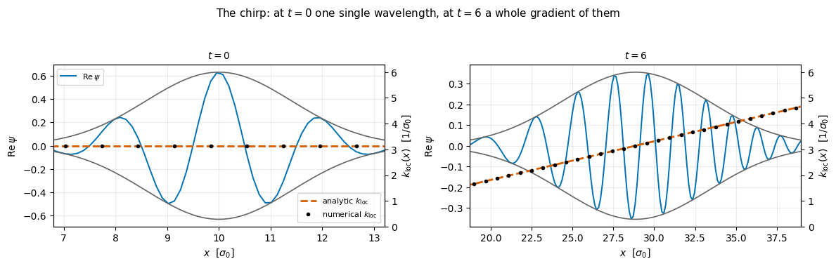
(b) The chirp. The imaginary part of the exponent gives a phase that is quadratic in \(X\):

\[ \theta(x,t) = k_0x - \frac{k_0^{2}t}{2} + \frac{\tau\,X^{2}}{4\sigma_0^{2}(1+\tau^{2})} - \frac12\arctan\tau . \]

The local wave number is its gradient,

\[ k_{\rm loc}(x,t) = \frac{\partial\theta}{\partial x} = k_0 + \frac{t\,X}{4\sigma_0^{2}\sigma^{2}(t)} \;\xrightarrow[t\gg t_s]{}\; k_0 + \frac{X}{t} . \]

Read that last formula aloud: at long times, the part of the packet sitting a distance \(X\) ahead of the centre is precisely the part whose velocity is \(X/t\) — it got there because it was moving that fast. The packet sorts itself in space by velocity, exactly like runners after the start of a race. In optics the same phenomenon is called a chirp (the instantaneous frequency sweeps across the pulse), and we will see it in an animation of \(\mathrm{Re}\,\psi\): the oscillations are stretched on one side and compressed on the other.

(c) The uncertainty product. Since \(\sigma_k\) is frozen and \(\sigma(t)\) grows,

\[ \sigma_x(t)\,\sigma_k = \frac12\sqrt{1+\tau^{2}} \;\ge\; \frac12 , \]

with equality only at \(t=0\). A free packet is a minimum-uncertainty state for one instant and never again. The bound itself is Heisenberg’s uncertainty relation [7]; the inequality \(\sigma_x\sigma_p \ge \hbar/2\) in this standard-deviation form was proved in [8].

(d) Phase velocity versus group velocity. A single plane wave \(e^{i(kx-\omega t)}\) with \(\omega = k^2/2\) has

\[ v_{\rm phase} = \frac{\omega}{k} = \frac{k}{2} , \qquad v_{\rm group} = \frac{d\omega}{dk} = k . \]

The envelope travels at \(k_0\); the ripples inside it travel at only \(k_0/2\), so in an animation of \(\mathrm{Re}\,\psi\) the individual crests continuously fall behind the lump and disappear at its rear edge. For light in vacuum the two velocities coincide; for matter waves they differ by a factor of two. The particle velocity of a de Broglie matter wave [9] is the group velocity, the one that carries the probability.

Physics insight. Everything above came from one fact: \(\omega(k)\) is not linear in \(k\). A linear dispersion (light in vacuum, sound in air) transports any pulse shape rigidly and forever. A curved \(\omega(k)\) makes pulses spread. In Section 6 we will discover that a careless discretisation changes \(\omega(k)\) — and therefore changes the physics.

4. Putting the problem on a grid

4.1 A grid, and what an array holds

A computer cannot hold a function \(\psi(x)\) — that is an uncountable infinity of numbers. It holds a finite array. So we choose a finite interval \([0, L)\) and \(N_x\) equally spaced points on it,

\[ x_j = j\,\Delta x, \qquad j = 0,1,\ldots,N_x-1, \qquad \Delta x = \frac{L}{N_x} , \]

and we store the \(N_x\) complex numbers

\[ \psi_j \;\equiv\; \psi(x_j) . \]

That is all a “state” is in this notebook: psi is a NumPy/JAX array of shape (N_x,) and dtype complex128, whose entry psi[j] is the value of the wave function at x[j]. The two knobs are \(L\) (how much of the world we keep) and \(\Delta x\) (how finely we resolve it), and the two errors they cause — boundary effects and discretisation error — are the two things we will have to control.

4.2 Integrals become sums

Every quantity we want is an integral, and every integral becomes a sum. For a smooth function sampled on a uniform grid, the Riemann sum (here: the left-endpoint rectangle rule — we sample at \(x_j = j\Delta x\) and weight every sample by \(\Delta x\). For a periodic function it is the trapezoidal rule: the trapezoidal rule would give the endpoints \(x_0\) and \(x_{N_x}\) half weight each, and on a ring those two points are the same point, so the two halves add up to one full \(\Delta x\)) reads

\[ \int_0^L f(x)\, dx \;\approx\; \Delta x \sum_{j=0}^{N_x-1} f(x_j) . \]

So the three quantities we care about are

\[ \mathcal{N} = \int \vert\psi\vert^{2} dx \;\to\; \Delta x \sum_j \vert\psi_j\vert^{2} , \qquad \langle x\rangle = \int x\,\vert\psi\vert^{2} dx \;\to\; \Delta x \sum_j x_j \vert\psi_j\vert^{2} , \]

\[ \sigma^{2} = \int (x - \langle x\rangle)^{2}\vert\psi\vert^{2} dx \;\to\; \Delta x \sum_j (x_j - \langle x\rangle)^{2}\,\vert\psi_j\vert^{2} . \]

For a periodic and smooth function this approximation is spectacularly good — the error decreases faster than any power of \(\Delta x\) (this is the trapezoidal rule’s superpower on periodic functions; see [10]). We will verify it numerically in a moment.

4.3 Periodic boundary conditions: the particle lives on a ring

What happens at \(x = 0\) and \(x = L\)? We impose periodic boundary conditions:

\[ \psi(x + L, t) = \psi(x, t) \qquad \Longleftrightarrow \qquad \psi_{N_x} \equiv \psi_0 . \]

Physically, periodic boundary conditions describe a particle confined to a ring of circumference \(L\), free to slide around it. Cold atoms are routinely trapped in exactly such ring geometries.

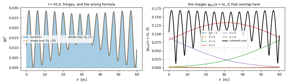
Numerically it is also the most convenient choice: there are no walls, so nothing reflects, and the translational symmetry survives — which, as Section 6.2 will show, makes plane waves exact eigenstates of the discretised Hamiltonian and hands us a very fast and very accurate algorithm. Its price is that a packet which runs off the right edge comes back in on the left. As long as the packet is narrow and stays far from the seam, the ring is indistinguishable from the infinite line; when it is not, the physics genuinely changes (Section 11).

4.4 The wave numbers that fit on a ring

A plane wave \(e^{ikx}\) is periodic with period \(L\) only if \(e^{ikL}=1\), that is

\[ k_n = \frac{2\pi n}{L}, \qquad n \in \mathbb{Z} . \]

On a grid of \(N_x\) points there are exactly \(N_x\) distinguishable such waves, conventionally taken as \(n = -N_x/2, \ldots, N_x/2-1\), because \(e^{i k_{n+N_x} x_j} = e^{ik_n x_j}e^{2\pi i j} = e^{ik_n x_j}\): the grid cannot tell \(n\) from \(n+N_x\). The largest wave number the grid represents is therefore

\[ k_{\max} = \frac{\pi}{\Delta x} \qquad \text{(the Nyquist wave number)} , \]

which is the sampling theorem proved in [11], the critical rate being named after Nyquist [12]: you need at least two grid points per wavelength. Two practical rules follow, and violating either of them is a common mistake:

1. Choose \(k_0\) commensurate with the ring, \(k_0 = 2\pi m/L\) with integer \(m\). Otherwise \(e^{ik_0x}\) is not periodic, and the initial state has a discontinuity at the seam \(x = L \equiv 0\).
2. Keep the whole packet inside the band: \(k_0 + \text{a few}\,\sigma_k \ll \pi/\Delta x\). Otherwise the high-\(k\) components are aliased — the grid silently reads a mode index \(m\) as \(m - N_x\), and as soon as \(m > N_x/2\) that is negative, so the component travels backwards.

Section 5.1 demonstrates both failures deliberately.

4.5 fftfreq: the order the wave numbers come in

NumPy’s fft, an implementation of the fast Fourier transform algorithm introduced in [13], returns the coefficients in the order \(n = 0, 1, \ldots, N_x/2-1, -N_x/2, \ldots, -1\) — the non-negative frequencies first, then the negative ones (“wrapped” order). Rather than remembering that, call np.fft.fftfreq(N_x, d=dx), which returns \(n/(N_x\Delta x) = n/L\) in exactly the matching order; multiply by \(2\pi\) to get \(k\):

k = 2.0 * np.pi * np.fft.fftfreq(N_x, d=dx)

Let us build the grid and look at it.

Code

# ==============================================================================
# STEP 1: the grid and the wave numbers it can represent
# ==============================================================================
def make_grid(L, N_x):
    """Uniform periodic grid on [0, L) and the matching FFT wave numbers.

    MATH
        x_j = j dx,  j = 0..N_x-1,  dx = L / N_x          (the ring [0,L) with x=L identified with x=0)
        k_n = 2 pi n / L,  n = 0,1,..,N_x/2-1,-N_x/2,..,-1  (the order produced by np.fft.fft)
    IMPLEMENTATION
        np.fft.fftfreq(N_x, d=dx) returns n / (N_x dx) = n / L in that same wrapped order.
    """
    dx = L / N_x
    x = np.arange(N_x) * dx                       # NOTE: the point x = L is NOT included (it is x = 0)
    k = 2.0 * np.pi * np.fft.fftfreq(N_x, d=dx)   # same length, same order as np.fft.fft(psi)
    return x, k, dx


# a small grid, so that we can print every single number
x_demo, k_demo, dx_demo = make_grid(L=8.0, N_x=8)
print("L = 8, N_x = 8  ->  dx =", dx_demo)
print("x =", x_demo)
print("k =", np.round(k_demo, 4), "   (in units of 2*pi/L:", np.round(k_demo * 8.0 / (2 * np.pi), 1), ")")
print(f"Nyquist wave number pi/dx = {np.pi / dx_demo:.4f}  = largest |k| on the grid")

L = 8, N_x = 8  ->  dx = 1.0
x = [0. 1. 2. 3. 4. 5. 6. 7.]
k = [ 0.      0.7854  1.5708  2.3562 -3.1416 -2.3562 -1.5708 -0.7854]    (in units of 2*pi/L: [ 0.  1.  2.  3. -4. -3. -2. -1.] )
Nyquist wave number pi/dx = 3.1416  = largest |k| on the grid

The printout shows the structure once and for all: eight positions \(0, 1, \ldots, 7\) (the ninth, \(x=8\), is \(x=0\)), and eight wave numbers in units of \(2\pi/L\): \(0,1,2,3,-4,-3,-2,-1\). The “wrap” after \(n=3\) is the wrapped ordering, and \(\vert k\vert_{\max} = 4\cdot 2\pi/8 = \pi = \pi/\Delta x\), as stated above.

4.6 The parameters of the main experiment

Now the real grid. We pick a ring of circumference \(L = 60\) (in units of \(\sigma_0\)) with \(N_x = 512\) points, a packet of width \(\sigma_0 = 1\) starting at \(x_c = 10\), and a kick \(k_0 = 2\pi\cdot 30/L = \pi\). Check the two rules: \(k_0\) is commensurate by construction, and \(\pi/\Delta x \approx 26.8\) is far above \(k_0 + 4\sigma_k = \pi + 2 \approx 5.1\). We will run to \(t_{\max} = 8\), by which time the centre has moved \(k_0 t = 25.1\) and the width has grown to \(\sigma = \sqrt{1+16} \approx 4.1\) — still comfortably inside the ring.

Code

# ==============================================================================
# PARAMETERS of the main experiment  (change them and re-run the notebook)
# ==============================================================================
L      = 60.0      # circumference of the ring          [units of sigma_0]
N_X    = 512       # number of grid points              [-]
SIGMA0 = 1.0       # initial width of the DENSITY       [units of sigma_0] -- = 1 by our choice of units
X_C    = 10.0      # initial centre of the packet       [units of sigma_0]
M0     = 30        # integer mode index of the kick: k0 = 2 pi M0 / L   (commensurate by construction)
T_MAX  = 8.0       # final time of the main run         [units of t_0]

K0 = 2.0 * np.pi * M0 / L                    # central wave number of the packet
SIGMA_K = 1.0 / (2.0 * SIGMA0)               # width of the momentum distribution (Section 3.2)

x, k, dx = make_grid(L, N_X)

print(f"grid      : L = {L}, N_x = {N_X}, dx = {dx:.6f}")
print(f"packet    : sigma_0 = {SIGMA0}, x_c = {X_C}, k_0 = 2*pi*{M0}/L = {K0:.6f}, sigma_k = {SIGMA_K}")
print(f"time scale: spreading time t_s = 2*sigma_0^2 = {2 * SIGMA0 ** 2:.3f},  run to t_max = {T_MAX}")
print()
print(f"RULE 1 (commensurate k0): k0*L/(2*pi) = {K0 * L / (2 * np.pi):.6f}  -> an integer, good")
print(f"RULE 2 (sampling)       : k0 + 4*sigma_k = {K0 + 4 * SIGMA_K:.3f}  must be << pi/dx = {np.pi / dx:.3f}"
      f"   -> ratio {(K0 + 4 * SIGMA_K) / (np.pi / dx):.3f}, good")
print(f"packet at t_max         : <x> = {X_C + K0 * T_MAX:.2f},  sigma = "
      f"{SIGMA0 * np.sqrt(1 + (T_MAX / (2 * SIGMA0 ** 2)) ** 2):.2f}  -> fits in [0, {L})")

grid      : L = 60.0, N_x = 512, dx = 0.117188
packet    : sigma_0 = 1.0, x_c = 10.0, k_0 = 2*pi*30/L = 3.141593, sigma_k = 0.5
time scale: spreading time t_s = 2*sigma_0^2 = 2.000,  run to t_max = 8.0

RULE 1 (commensurate k0): k0*L/(2*pi) = 30.000000  -> an integer, good
RULE 2 (sampling)       : k0 + 4*sigma_k = 5.142  must be << pi/dx = 26.808   -> ratio 0.192, good
packet at t_max         : <x> = 35.13,  sigma = 4.12  -> fits in [0, 60.0)

5. First contact: build the packet and measure it

We now write the two functions that encode Section 3 — the initial state, Eq. (3), and the exact solution, Eq. (7) — and the three “measurement” functions that turn an array into physics, following Section 4.2.

Two remarks on the measurement functions:

• They are written for a ring, so the mean position needs care: the naive \(\sum_j x_j\vert\psi_j\vert^2\) is meaningless for a packet sitting on top of the seam (half of it at \(x\approx 0\), half at \(x\approx L\), mean \(\approx L/2\) — the opposite side of the ring). The standard fix is the circular mean: map each point to the unit circle, \(x_j \mapsto e^{2\pi i x_j/L}\), average, and read off the angle. For a packet symmetric about its centre (our Gaussian) this returns the ordinary mean, and it keeps working when the packet crosses the seam.
• The width is then measured with the wrapped distance to that mean, \(d_j = \big((x_j - \bar x + L/2) \bmod L\big) - L/2\), which is the shortest way around the ring.

Code

# ==============================================================================
# STEP 2: the physics, as five short functions
# ==============================================================================
def gaussian_packet(x, x_c, sigma0, k0):
    """Initial Gaussian wave packet with an imprinted momentum -- Eq. (3).

    MATH
        psi(x,0) = (2 pi sigma0^2)^(-1/4) exp(-(x-x_c)^2 / (4 sigma0^2)) exp(i k0 x)
        |psi|^2 is a normal density of standard deviation sigma0 centred at x_c.
    """
    envelope = np.exp(-(x - x_c) ** 2 / (4.0 * sigma0 ** 2))
    carrier = np.exp(1j * k0 * x)                      # pure phase: does NOT change |psi|^2
    return ((2.0 * np.pi * sigma0 ** 2) ** (-0.25) * envelope * carrier).astype(CDTYPE)


def psi_exact_line(x, t, x_c, sigma0, k0):
    """Exact solution on the INFINITE LINE -- Eq. (7).

    MATH
        tau = t / (2 sigma0^2),   X = x - x_c - k0 t
        psi = (2 pi sigma0^2)^(-1/4) / sqrt(1 + i tau)
              * exp(-X^2 / (4 sigma0^2 (1 + i tau)))
              * exp(i (k0 x - k0^2 t / 2))
    """
    tau = t / (2.0 * sigma0 ** 2)
    X = x - x_c - k0 * t                               # position in the frame moving with the packet
    prefactor = (2.0 * np.pi * sigma0 ** 2) ** (-0.25) / np.sqrt(1.0 + 1j * tau)
    envelope = np.exp(-X ** 2 / (4.0 * sigma0 ** 2 * (1.0 + 1j * tau)))
    carrier = np.exp(1j * (k0 * x - 0.5 * k0 ** 2 * t))
    return (prefactor * envelope * carrier).astype(CDTYPE)


def norm_riemann(psi, dx):
    """Norm squared:  N = integral |psi|^2 dx  ->  dx * sum_j |psi_j|^2."""
    return float(dx * np.sum(np.abs(psi) ** 2))


def mean_position(psi, x, dx, L):
    """Mean position on a RING, via the circular mean.

    MATH
        z = dx sum_j |psi_j|^2 exp(2 pi i x_j / L);   <x> = (L / 2 pi) * arg(z)  (mod L)
    IMPLEMENTATION
        For a packet symmetric about its centre and far from the seam this equals dx sum_j x_j |psi_j|^2
        (up to round-off), and it also survives a packet sitting on the seam x = 0 == L.
    """
    p = np.abs(psi) ** 2 * dx
    z = np.sum(p * np.exp(2j * np.pi * x / L))
    return float((np.angle(z) % (2.0 * np.pi)) * L / (2.0 * np.pi))


def packet_width(psi, x, dx, L):
    """Standard deviation of |psi|^2 on a ring, measured with the wrapped distance to the circular mean.

    MATH
        d_j = ((x_j - <x> + L/2) mod L) - L/2      (shortest signed distance on the ring)
        sigma^2 = sum_j d_j^2 |psi_j|^2 dx / sum_j |psi_j|^2 dx
    """
    p = np.abs(psi) ** 2 * dx
    d = (x - mean_position(psi, x, dx, L) + 0.5 * L) % L - 0.5 * L
    return float(np.sqrt(np.sum(p * d ** 2) / np.sum(p)))


# ------------------------------------------------------------------------------
# Build the initial state and measure it -- the very first numbers of the course
# ------------------------------------------------------------------------------
psi0 = gaussian_packet(x, X_C, SIGMA0, K0)

print("psi0 is an array:", type(psi0).__name__, psi0.shape, psi0.dtype)
print(f"norm   dx*sum|psi|^2 = {norm_riemann(psi0, dx):.15f}   (exact value: 1)")
print(f"<x>                  = {mean_position(psi0, x, dx, L):.15f}   (exact value: {X_C})")
print(f"sigma                = {packet_width(psi0, x, dx, L):.15f}   (exact value: {SIGMA0})")

# CHECKPOINT: the Riemann sums must reproduce the analytic values to (nearly) machine precision,
# because |psi|^2 is smooth and periodic on the ring -- see Section 4.2.
assert abs(norm_riemann(psi0, dx) - 1.0) < 1e3 * TOL
assert abs(mean_position(psi0, x, dx, L) - X_C) < 1e3 * TOL
assert abs(packet_width(psi0, x, dx, L) - SIGMA0) < 1e3 * TOL
print("\nCHECKPOINT passed: sums reproduce integrals to ~1e-15.")

psi0 is an array: ndarray (512,) complex128
norm   dx*sum|psi|^2 = 1.000000000000000   (exact value: 1)
<x>                  = 9.999999999999998   (exact value: 10.0)
sigma                = 1.000000000000000   (exact value: 1.0)

CHECKPOINT passed: sums reproduce integrals to ~1e-15.

We replaced three integrals over the whole real line by three sums of \(512\) terms, and got the right answers to fifteen decimal places. That is the periodic trapezoidal rule at work: for a smooth function on a ring, the Riemann sum is extremely accurate. (For a non-periodic function the same left-endpoint sum is only \(O(\Delta x)\) accurate, and \(O(\Delta x^2)\) once the two end points get half weight.)

The one tiny discrepancy you do see, in the last digit of \(\langle x\rangle\), is round-off error: a float64 number carries about \(16\) significant decimal digits, so the smallest relative error any computation can have is \(\varepsilon \approx 2.2\times10^{-16}\), the machine epsilon. Summing \(512\) numbers accumulates a few of those. “Machine precision” in this course means: as accurate as double-precision arithmetic allows, i.e. a relative error of order \(10^{-16}\)–\(10^{-13}\). Nothing can ever be better than that, and a result at that level is exact for all practical purposes.

Now let us look at the packet.

Code

# ==============================================================================
# FIGURE: the initial state -- density, real part, and momentum distribution
# ==============================================================================
C_NUM, C_ANA, C_FD = "#0072B2", "#D55E00", "#009E73"      # colour-blind friendly: blue / orange / green

phi0 = np.fft.fft(psi0)                                    # coefficients of psi0 in the plane-wave basis
weights = np.abs(phi0) ** 2 / np.sum(np.abs(phi0) ** 2)    # normalised |phi(k)|^2 (the momentum distribution)
k_sorted = np.argsort(k)                                   # undo the wrapped ordering, for plotting only

fig, axes = plt.subplots(1, 3, figsize=(13.5, 3.4))

axes[0].fill_between(x, 0, np.abs(psi0) ** 2, color=C_NUM, alpha=0.4)
axes[0].plot(x, np.abs(psi0) ** 2, color=C_NUM, lw=1.8)
axes[0].axvline(X_C, color="k", ls=":", lw=1)
axes[0].set_xlabel(r"$x$  [$\sigma_0$]"), axes[0].set_ylabel(r"$|\psi(x,0)|^2$")
axes[0].set_title(r"density: a lump of width $\sigma_0$")

axes[1].plot(x, psi0.real, color=C_NUM, lw=1.2, label=r"$\mathrm{Re}\,\psi$")
axes[1].plot(x, np.abs(psi0), color="k", lw=1.4, ls="--", label=r"$|\psi|$ (envelope)")
axes[1].plot(x, -np.abs(psi0), color="k", lw=1.4, ls="--")
axes[1].set_xlim(X_C - 5, X_C + 5)
axes[1].set_xlabel(r"$x$  [$\sigma_0$]"), axes[1].set_ylabel(r"$\mathrm{Re}\,\psi(x,0)$")
axes[1].set_title(r"the carrier $e^{ik_0x}$ under the envelope")
axes[1].legend(fontsize=8, loc="upper right")

axes[2].plot(k[k_sorted], weights[k_sorted] / (2 * np.pi / L), color=C_NUM, lw=1.8, label="numerics")
k_fine = np.linspace(-8, 8, 400)
axes[2].plot(k_fine, np.exp(-2 * SIGMA0 ** 2 * (k_fine - K0) ** 2) / np.sqrt(np.pi / (2 * SIGMA0 ** 2)),
             color=C_ANA, ls="--", lw=1.6, label="analytic, Eq. (5)")
axes[2].axvline(K0, color="k", ls=":", lw=1)
axes[2].set_xlim(-8, 8)
axes[2].set_xlabel(r"$k$  [$1/\sigma_0$]"), axes[2].set_ylabel(r"$|\phi(k)|^2$")
axes[2].set_title(r"momentum distribution, centred at $k_0$")
axes[2].legend(fontsize=8)

for ax in axes:
    ax.grid(alpha=0.25)
fig.suptitle("The initial Gaussian wave packet", y=1.04)
fig.tight_layout()
plt.show()

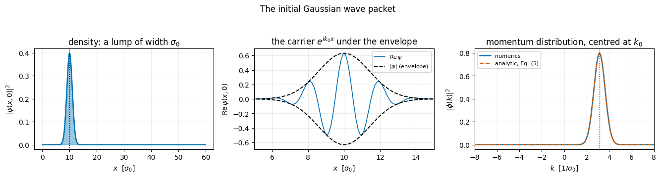
Left: the probability density — a bump of width \(\sigma_0 = 1\) at \(x_c = 10\), and zero (to machine precision) everywhere else, in particular at the seam. Middle: zoomed in, the real part of \(\psi\) oscillates under the Gaussian envelope with wavelength \(2\pi/k_0 = 2\); this carrier is the momentum. Right: the momentum distribution obtained from the FFT of the array, on top of the analytic Gaussian of Eq. (5) centred at \(k_0 = \pi\) with width \(\sigma_k = 0.5\). The two curves lie on top of each other — our first numerics-versus-analytics comparison, and the FFT has just passed its first test.

5.1 The two rules of Section 4.4, violated on purpose

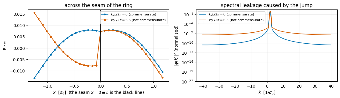
Rule 1: a non-commensurate \(k_0\). If \(k_0 L/(2\pi)\) is not an integer, \(e^{ik_0x}\) jumps at the seam. For our narrow packet the wave function there is \(\sim e^{-25}\), so nothing happens — but as soon as the packet is wide enough to reach the boundary, the jump is a real discontinuity, and a discontinuity in \(x\) means a fat tail in \(k\) (“spectral leakage”) which the grid cannot represent. Let us make a deliberately wide packet and look.

Rule 2: aliasing. The grid cannot tell the mode index \(m\) from \(m + N_x\): the two sampled arrays are the same array, because \(e^{i2\pi(m+N_x)x_j/L} = e^{i2\pi m x_j/L}\,e^{2\pi i j}\) and \(e^{2\pi ij}=1\). So the grid always reports the index in the band, i.e. \(m\) reduced modulo \(N_x\) into \([-N_x/2, N_x/2)\). And that is the trap: if we ask for \(m\) with \(N_x/2 < m < N_x\), the grid reads it as \(m - N_x < 0\), and the packet we think we kicked to the right calmly travels to the left. The next cell checks both statements on arrays.

Code

# ==============================================================================
# FAILURE DEMO 1: k0 not commensurate with the ring  ->  a jump at the seam
# FAILURE DEMO 2: k0 above the Nyquist limit         ->  aliasing (the packet turns around)
# ==============================================================================
# --- Demo 1: a wide packet (sigma = 2.5) on a small ring, with and without commensurate k0 ---
L_w, N_w = 20.0, 256
x_w, k_w, dx_w = make_grid(L_w, N_w)
psi_good = gaussian_packet(x_w, 0.5 * L_w, 2.5, 2.0 * np.pi * 6 / L_w)     # m = 6      (commensurate)
psi_bad = gaussian_packet(x_w, 0.5 * L_w, 2.5, 2.0 * np.pi * 6.5 / L_w)   # m = 6.5    (NOT commensurate)

fig, axes = plt.subplots(1, 2, figsize=(11.5, 3.4))
for psi_c, lab, col, ls in ((psi_good, r"$k_0 L/2\pi = 6$ (commensurate)", C_NUM, "-"),
                            (psi_bad, r"$k_0 L/2\pi = 6.5$ (not commensurate)", C_ANA, "-")):
    # roll the array so that the seam x = 0 == L sits in the middle of the picture
    axes[0].plot(np.concatenate([x_w - L_w, x_w])[N_w - 16:N_w + 16],
                 np.concatenate([psi_c.real, psi_c.real])[N_w - 16:N_w + 16], ls + "o", color=col, lw=1.6,
                 ms=3.5, label=lab)
    w = np.abs(np.fft.fft(psi_c)) ** 2
    axes[1].semilogy(k_w[np.argsort(k_w)], (w / w.max())[np.argsort(k_w)], color=col, lw=1.4, label=lab)
axes[0].axvline(0.0, color="k", lw=1.2)
axes[0].set_xlabel(r"$x$  [$\sigma_0$]  (the seam $x=0\equiv L$ is the black line)")
axes[0].set_ylabel(r"$\mathrm{Re}\,\psi$")
axes[0].set_title("across the seam of the ring")
axes[1].set_xlabel(r"$k$  [$1/\sigma_0$]"), axes[1].set_ylabel(r"$|\phi(k)|^2$ (normalised)")
axes[1].set_ylim(1e-22, 3), axes[1].set_title("spectral leakage caused by the jump")
for ax in axes:
    ax.grid(alpha=0.25), ax.legend(fontsize=8)
fig.tight_layout()
plt.show()

# --- Demo 2: aliasing is exact, not approximate ---
m_ok = N_X // 2 - 20                      # a legal mode index
m_alias = m_ok + N_X                      # the SAME grid function, N_x modes higher
psi_a = gaussian_packet(x, X_C, SIGMA0, 2.0 * np.pi * m_ok / L)
psi_b = gaussian_packet(x, X_C, SIGMA0, 2.0 * np.pi * m_alias / L)
print(f"k0 for m = {m_ok:5d}:  {2 * np.pi * m_ok / L:8.4f}   (inside the band, |k| < pi/dx = {np.pi / dx:.3f})")
print(f"k0 for m = {m_alias:5d}:  {2 * np.pi * m_alias / L:8.4f}   (far outside the band)")
print(f"max |psi_a - psi_b| on the grid = {np.max(np.abs(psi_a - psi_b)):.3e}"
      "   <- the grid cannot tell them apart (this is round-off, the two arrays are the SAME function)")
assert np.max(np.abs(psi_a - psi_b)) < 1e4 * TOL

# ... and the consequence: an index just ABOVE N_x/2 is read as a NEGATIVE one, i.e. as a kick to the LEFT
m_right = N_X // 2 + 40                   # we *think* we kick to the right with k0 = 2 pi m_right / L
m_seen = m_right - N_X                    # what the grid actually holds: a negative mode index
psi_r = gaussian_packet(x, X_C, SIGMA0, 2.0 * np.pi * m_right / L)
psi_l = gaussian_packet(x, X_C, SIGMA0, 2.0 * np.pi * m_seen / L)
w_r = np.abs(np.fft.fft(psi_r)) ** 2
print(f"\nwe ask for m = {m_right} -> k0 = {2 * np.pi * m_right / L:+8.4f}  (above Nyquist pi/dx = {np.pi / dx:.3f})")
print(f"the grid stores m = {m_seen} -> k0 = {2 * np.pi * m_seen / L:+8.4f}  <- NEGATIVE: the packet will move LEFT")
print(f"   max |psi(m={m_right}) - psi(m={m_seen})| = {np.max(np.abs(psi_r - psi_l)):.3e}   (the same array)")
print(f"   <k> read back from the array           = {np.sum(w_r * k) / np.sum(w_r):+8.4f}"
      f"   (requested: {2 * np.pi * m_right / L:+.4f})")
assert np.sum(w_r * k) / np.sum(w_r) < 0.0, "an over-Nyquist kick is read back as a negative momentum"

k0 for m =   236:   24.7139   (inside the band, |k| < pi/dx = 26.808)
k0 for m =   748:   78.3304   (far outside the band)
max |psi_a - psi_b| on the grid = 4.019e-14   <- the grid cannot tell them apart (this is round-off, the two arrays are the SAME function)

we ask for m = 296 -> k0 = +30.9970  (above Nyquist pi/dx = 26.808)
the grid stores m = -216 -> k0 = -22.6195  <- NEGATIVE: the packet will move LEFT
   max |psi(m=296) - psi(m=-216)| = 2.223e-14   (the same array)
   <k> read back from the array           = -22.6195   (requested: +30.9970)

Left panel: the commensurate packet (blue) crosses the seam continuously; the non-commensurate one (orange) jumps — the value coming back in at \(x=0\) does not match the value leaving at \(x=L\).

Right panel: a discontinuity in real space is a fat tail in Fourier space. This deliberately wide packet (\(\sigma_0 = 2.5\) on a ring of only \(L=20\)) is not small at the seam either, so even the commensurate one has a tail — its slope is discontinuous there, which gives \(\vert\phi\vert^2 \sim k^{-4}\) and a floor near \(10^{-10}\) (blue). The non-commensurate packet has a jump in the value, which gives only \(\vert\phi\vert^2 \sim k^{-2}\) and a floor a thousand times higher (orange). Those components are not physics; they are the seam, and at the edge of the band they get aliased. Always choose \(k_0 = 2\pi m/L\) with integer \(m\) — and keep the packet away from the seam, or accept that you are simulating a genuinely different initial state.

The aliasing print: two wave numbers differing by \(N_x\) modes give the same grid function — the printed \(10^{-14}\) is only the round-off of evaluating two different exp expressions, not a physical difference. There is no approximation here and no warning message; the information is simply not on the grid. The second half of the print makes the damage concrete: asking for the mode index \(m = N_x/2 + 40\) stores the array of \(m - N_x = -216\), and reading the mean momentum back off that array returns a negative number. The packet will move to the left. If you ever see a packet moving in the wrong direction, check \(k_0\) against \(\pi/\Delta x\) first.

6. Method A — finite differences

We now need the second derivative of an array. This is the first genuinely numerical idea of the course.

6.1 Deriving the three-point Laplacian

Taylor-expand the exact function around \(x_j\), in both directions, to fourth order:

\[ \begin{aligned} \psi(x_j+\Delta x) &= \psi_j + \Delta x\,\psi'_j + \tfrac{\Delta x^{2}}{2}\psi''_j + \tfrac{\Delta x^{3}}{6}\psi'''_j + \tfrac{\Delta x^{4}}{24}\psi''''_j + \ldots \\ \psi(x_j-\Delta x) &= \psi_j - \Delta x\,\psi'_j + \tfrac{\Delta x^{2}}{2}\psi''_j - \tfrac{\Delta x^{3}}{6}\psi'''_j + \tfrac{\Delta x^{4}}{24}\psi''''_j - \ldots \end{aligned} \]

Add the two lines. The odd derivatives cancel, and

\[ \psi_{j+1} + \psi_{j-1} = 2\psi_j + \Delta x^{2}\psi''_j + \frac{\Delta x^{4}}{12}\psi''''_j + O(\Delta x^{6}) . \]

Solve for \(\psi''_j\):

\[ \boxed{\;\psi''_j \;=\; \frac{\psi_{j+1} - 2\psi_j + \psi_{j-1}}{\Delta x^{2}} \;-\; \frac{\Delta x^{2}}{12}\psi''''_j + O(\Delta x^{4}) \;} \tag{9} \]

The first term is the three-point Laplacian; the rest is the discretisation error, which is \(O(\Delta x^2)\): the method is second-order accurate. Halving \(\Delta x\) divides the error by four. That prediction is testable, and we will test it.

On the ring, “\(j+1\)” for \(j = N_x-1\) means \(j=0\): the stencil wraps around. In NumPy this is one line, np.roll(psi, -1) - 2*psi + np.roll(psi, +1), with no loop and no special treatment of the edges.

6.2 The Hamiltonian is a circulant matrix

Writing \(H = -\tfrac12 \partial_x^2\) with the stencil (9) gives a matrix acting on the vector \((\psi_0,\ldots,\psi_{N_x-1})\):

\[ H_{jl} = \frac{1}{2\Delta x^{2}}\left(2\delta_{j,l} - \delta_{j,l+1} - \delta_{j,l-1}\right), \qquad \text{indices mod } N_x . \]

Every row is the previous row shifted by one — a circulant matrix. That single structural fact is the key to everything in this section and the next, because of a classical theorem:

The eigenvectors of any circulant matrix are the plane waves \(v^{(n)}_j = e^{ik_nx_j}/\sqrt{N_x}\), whatever the entries are. Only the eigenvalues depend on them.

The reason is symmetry: a circulant matrix commutes with the shift \(j \to j+1\), and the plane waves are the eigenvectors of the shift. Let us find the eigenvalues by simply applying \(H\) to a plane wave:

\[ \begin{aligned} \left(H v^{(n)}\right)_j &= \frac{1}{2\Delta x^{2}} \left(2 e^{ik_nx_j} - e^{ik_nx_{j+1}} - e^{ik_nx_{j-1}}\right) \frac{1}{\sqrt{N_x}} \\ &= \frac{e^{ik_nx_j}}{2\Delta x^{2}\sqrt{N_x}}\left(2 - e^{ik_n\Delta x} - e^{-ik_n\Delta x}\right) = \frac{1 - \cos(k_n\Delta x)}{\Delta x^{2}}\; v^{(n)}_j , \end{aligned} \]

using \(e^{i\theta}+e^{-i\theta} = 2\cos\theta\). So the discrete dispersion relation is

\[ \boxed{\;\omega_{\rm FD}(k) \;=\; \frac{1-\cos(k\Delta x)}{\Delta x^{2}}\;} \qquad\text{versus the exact}\qquad \omega(k) = \frac{k^{2}}{2} . \tag{10} \]

Expand for small \(k\Delta x\), using \(\cos\theta = 1 - \theta^2/2 + \theta^4/24 - \ldots\):

\[ \omega_{\rm FD}(k) = \frac{k^{2}}{2} - \frac{k^{4}\Delta x^{2}}{24} + O(\Delta x^{4}) , \]

confirming the \(O(\Delta x^2)\) accuracy of Eq. (9), and showing exactly how the discretisation lies: it makes high-\(k\) components too slow. The group velocity of the discretised theory is

\[ v_{\rm FD}(k) = \frac{d\omega_{\rm FD}}{dk} = \frac{\sin(k\Delta x)}{\Delta x} \;<\; k \qquad (0 < k \le \pi/\Delta x) , \]

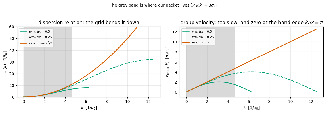
since \(\sin\theta<\theta\) for \(\theta>0\). Worse than “too slow”: \(v_{\rm FD}\) is not even monotonic. It rises to a maximum \(1/\Delta x\) at \(k\Delta x = \pi/2\) and then falls back, reaching exactly zero at the edge of the band, \(k\Delta x = \pi\). The fastest-oscillating grid modes — those with two points per wavelength — do not propagate at all in the finite-difference model, although the true theory says they are the fastest of all. (They are also exactly the modes the grid barely resolves, so the two failures arrive together.)

6.3 The exact propagator of the discretised Hamiltonian

Because we know all the eigenvectors and eigenvalues of \(H_{\rm FD}\), we can apply \(e^{-iH_{\rm FD}t}\) exactly, with no time step and no time-integration error at all:

1. expand \(\psi\) in plane waves (that is what the FFT does): \(\phi_n = \mathrm{FFT}[\psi]_n\);
2. multiply each coefficient by \(e^{-i\omega_{\rm FD}(k_n) t}\);
3. transform back with the inverse FFT.

This is a deliberate choice: it isolates the spatial discretisation error, which is what we want to study.

Code

# ==============================================================================
# STEP 3: the finite-difference Hamiltonian as an explicit matrix (small N_x only)
#   We build it once, for N_x = 8, to SEE the circulant structure and to CHECK
#   the eigenvalue formula (10).  For production we never build this matrix.
# ==============================================================================
def fd_hamiltonian_matrix(N_x, dx):
    """Dense matrix of H = -(1/2) d^2/dx^2 with the 3-point stencil and periodic wrap-around.

    MATH
        H[j,l] = (2 delta_{j,l} - delta_{j,l+1} - delta_{j,l-1}) / (2 dx^2),  indices modulo N_x
    COST
        N_x^2 memory -- this is a TEACHING function; the production code never forms H.
    """
    H = np.zeros((N_x, N_x))
    for j in range(N_x):
        H[j, j] = 2.0
        H[j, (j + 1) % N_x] = -1.0                 # the "% N_x" IS the periodic boundary condition
        H[j, (j - 1) % N_x] = -1.0
    return H / (2.0 * dx ** 2)


H_small = fd_hamiltonian_matrix(8, 1.0)            # dx = 1 so the numbers are readable
print("H for N_x = 8, dx = 1  (every row is the row above, shifted by one -> CIRCULANT):")
print(H_small)
print("\nnote the two entries in the corners: they connect site 7 to site 0 -- the ring closes here.")

# CHECKPOINT: the eigenvalues must be (1 - cos(k dx)) / dx^2 -- Eq. (10)
x8, k8, dx8 = make_grid(L=8.0, N_x=8)
eigenvalues_numeric = np.sort(np.linalg.eigvalsh(H_small))
eigenvalues_formula = np.sort((1.0 - np.cos(k8 * dx8)) / dx8 ** 2)
print(f"\neigenvalues from numpy  : {np.round(eigenvalues_numeric, 6)}")
print(f"eigenvalues from Eq.(10): {np.round(eigenvalues_formula, 6)}")
err_eig = float(np.max(np.abs(eigenvalues_numeric - eigenvalues_formula)))
print(f"max difference = {err_eig:.3e}")
assert err_eig < 1e4 * TOL
print("CHECKPOINT passed: plane waves really are the eigenvectors of the finite-difference Hamiltonian.")

H for N_x = 8, dx = 1  (every row is the row above, shifted by one -> CIRCULANT):
[[ 1.  -0.5  0.   0.   0.   0.   0.  -0.5]
 [-0.5  1.  -0.5  0.   0.   0.   0.   0. ]
 [ 0.  -0.5  1.  -0.5  0.   0.   0.   0. ]
 [ 0.   0.  -0.5  1.  -0.5  0.   0.   0. ]
 [ 0.   0.   0.  -0.5  1.  -0.5  0.   0. ]
 [ 0.   0.   0.   0.  -0.5  1.  -0.5  0. ]
 [ 0.   0.   0.   0.   0.  -0.5  1.  -0.5]
 [-0.5  0.   0.   0.   0.   0.  -0.5  1. ]]

note the two entries in the corners: they connect site 7 to site 0 -- the ring closes here.

eigenvalues from numpy  : [-0.        0.292893  0.292893  1.        1.        1.707107  1.707107
  2.      ]
eigenvalues from Eq.(10): [0.       0.292893 0.292893 1.       1.       1.707107 1.707107 2.      ]
max difference = 5.551e-16
CHECKPOINT passed: plane waves really are the eigenvectors of the finite-difference Hamiltonian.

The matrix is exactly as advertised: \(2\) on the diagonal, \(-1\) next to it, and a \(-1\) in the two far corners, H[0, 7] and H[7, 0], which is where the ring closes. Its eigenvalues agree with the closed-form expression (10) to machine precision, which confirms the whole algebra of Section 6.2.

Now let us plot the two dispersion relations against each other. This single figure explains every finite-difference error we will see later.

Code

# ==============================================================================
# FIGURE: exact versus discrete dispersion relation, and the group velocities
# ==============================================================================
fig, axes = plt.subplots(1, 2, figsize=(11.5, 3.8))
for dx_test, style in ((0.5, "-"), (0.25, "--")):
    kk = np.linspace(0, np.pi / dx_test, 400)
    axes[0].plot(kk, (1 - np.cos(kk * dx_test)) / dx_test ** 2, style, color=C_FD, lw=1.8,
                 label=rf"$\omega_{{\rm FD}}$, $\Delta x = {dx_test}$")
    axes[1].plot(kk, np.sin(kk * dx_test) / dx_test, style, color=C_FD, lw=1.8,
                 label=rf"$v_{{\rm FD}}$, $\Delta x = {dx_test}$")
kk = np.linspace(0, np.pi / 0.25, 400)
axes[0].plot(kk, 0.5 * kk ** 2, color=C_ANA, lw=2.0, label=r"exact $\omega = k^2/2$")
axes[1].plot(kk, kk, color=C_ANA, lw=2.0, label=r"exact $v = k$")
axes[0].axvspan(0, K0 + 3 * SIGMA_K, color="0.85", zorder=0)
axes[1].axvspan(0, K0 + 3 * SIGMA_K, color="0.85", zorder=0)
axes[0].set_ylim(0, 60), axes[1].set_ylim(-1, 13)
axes[1].axhline(0.0, color="k", lw=0.8)
axes[0].set_xlabel(r"$k$  [$1/\sigma_0$]"), axes[0].set_ylabel(r"$\omega(k)$  [$1/t_0$]")
axes[0].set_title("dispersion relation: the grid bends it down")
axes[1].set_xlabel(r"$k$  [$1/\sigma_0$]"), axes[1].set_ylabel(r"$v_{\rm group}(k)$  [$\sigma_0/t_0$]")
axes[1].set_title(r"group velocity: too slow, and zero at the band edge $k\Delta x = \pi$")
for ax in axes:
    ax.grid(alpha=0.25), ax.legend(fontsize=8, loc="upper left")
fig.suptitle(r"The grey band is where our packet lives ($k \lesssim k_0 + 3\sigma_k$)", y=1.03, fontsize=10)
fig.tight_layout()
plt.show()

Inside the grey band — where our packet actually has weight — the discrete curves hug the exact ones, and they hug them more closely for the finer grid: this is the \(O(\Delta x^2)\) of Eq. (9), visible to the eye. Towards the edge of the band the discretisation is simply a different physical theory: \(\omega_{\rm FD}\) saturates at \(2/\Delta x^2\) instead of growing like \(k^2\), and the group velocity, after peaking at \(1/\Delta x\), comes back down to zero. Each curve stops at its own Nyquist wave number \(\pi/\Delta x\) — there is nothing to plot beyond it, because the grid holds no such mode.

Common pitfall. A “converged-looking” finite-difference simulation can still be wrong if the state develops structure on the scale of \(\Delta x\) (sharp fronts, high-momentum components after hitting a barrier). The way to find out is to run two grids and compare.

7. Method B — the Fourier (spectral) method

Look again at Section 6.3: to apply \(e^{-iH_{\rm FD}t}\) we went to Fourier space, multiplied by a phase, and came back. The exact Hamiltonian is diagonal in Fourier space too, Eq. (6). So the very same three steps, with \(\omega_{\rm FD}\) replaced by the exact \(\omega = k^2/2\), solve the original equation:

\[ \boxed{\;\psi(x,t) \;=\; \mathrm{IFFT}\Big[\,e^{-i k^{2}t/2}\;\mathrm{FFT}\big[\psi(x,0)\big]\Big] \;} \tag{11} \]

This is the Fourier (spectral) method, and it has remarkable properties:

• it is exact in time — Eq. (11) holds for any \(t\), small or huge, with no time step at all;
• it is spectrally accurate in space — the only error is that the grid truncates the momentum band at \(\pi/\Delta x\), i.e. it throws away \(\vert\phi(k)\vert^2 \propto e^{-2\sigma_0^2(k-k_0)^2}\) for \(\vert k\vert>\pi/\Delta x\). By Parseval the \(L^2\) error is the square root of that discarded weight, so it falls like \(e^{-\sigma_0^{2}\left(\pi/\Delta x - k_0\right)^{2}}\): exponentially in \(1/\Delta x\), faster than any power. Compare with \(O(\Delta x^2)\);
• it costs \(O(N_x\log N_x)\) per application, thanks to the Fast Fourier Transform, versus \(O(N_x^2)\) for a dense matrix-vector product and \(O(N_x^3)\) for building a matrix exponential.

Fourier grid methods for wave-packet dynamics were introduced in [14] and [15]; Ref. [16] (Chapters 3–4) explains the exponential accuracy, and Ref. [17], Chapter 12, the FFT itself.

Everything rests on periodicity: the FFT assumes the array is one period of a periodic function. That is exactly the ring, so we pay nothing.

7.1 One function for both methods

Both methods have the identical form “FFT, multiply by \(e^{-i\omega(k)t}\), IFFT”; they differ only in the array \(\omega(k)\). So we write one propagator and feed it either dispersion relation. This is also our first JAX code.

JAX practice. jax.jit compiles a Python function once, for the given argument shapes, into a single optimised machine program, so the FFT, the multiplication and the inverse FFT run without Python overhead. jax.vmap(f) turns a function written for one input into one that handles a whole batch — here, all the snapshot times at once, without a Python loop. Both are explained properly in notebook 01, JAX; for now, read jnp as “NumPy”.

Code

# ==============================================================================
# STEP 4: THE propagator -- three lines that solve the Schrodinger equation
# ==============================================================================
@jax.jit
def propagate(psi, omega_k, t):
    """Exact evolution under any Hamiltonian that is diagonal in the plane-wave basis.

    MATH
        psi(t) = IFFT[ exp(-i omega(k) t) * FFT[psi(0)] ]
        omega(k) = k^2/2              -> the exact free Schrodinger equation      (spectral method)
        omega(k) = (1-cos(k dx))/dx^2 -> the 3-point finite-difference Hamiltonian (Eq. 10)
    IMPLEMENTATION
        psi and omega_k are arrays of shape (N_x,) in the SAME wrapped order as np.fft.fftfreq.
    COST
        O(N_x log N_x) per call, dominated by the two FFTs.  No time step: t may be any number.
    JAX
        jax.jit compiles the three operations into one program; t may be traced (a JAX scalar).
    """
    return jnp.fft.ifft(jnp.exp(-1j * omega_k * t) * jnp.fft.fft(psi))


# vmap over the LAST argument (t): one call -> a stack of snapshots, shape (n_times, N_x)
propagate_times = jax.jit(jax.vmap(propagate, in_axes=(None, None, 0)))

# the two dispersion relations, as arrays on our k-grid
omega_exact = jnp.asarray(0.5 * k ** 2, dtype=RDTYPE)                      # exact:  k^2/2
omega_fd = jnp.asarray((1.0 - np.cos(k * dx)) / dx ** 2, dtype=RDTYPE)     # 3-point stencil: Eq. (10)

psi0_j = jnp.asarray(psi0)                                                 # move the initial state to JAX
t_check = 3.0
psi_spec = np.asarray(propagate(psi0_j, omega_exact, t_check))
psi_fd = np.asarray(propagate(psi0_j, omega_fd, t_check))
psi_ana = psi_exact_line(x, t_check, X_C, SIGMA0, K0)

print(f"at t = {t_check}:")
print(f"  <x>  spectral = {mean_position(psi_spec, x, dx, L):.10f}   "
      f"FD = {mean_position(psi_fd, x, dx, L):.10f}   analytic = {X_C + K0 * t_check:.10f}")
print(f"  sigma spectral = {packet_width(psi_spec, x, dx, L):.10f}   "
      f"FD = {packet_width(psi_fd, x, dx, L):.10f}   analytic = "
      f"{SIGMA0 * np.sqrt(1 + (t_check / (2 * SIGMA0 ** 2)) ** 2):.10f}")
print(f"  max | |psi_spec|^2 - |psi_ana|^2 | = {np.max(np.abs(np.abs(psi_spec) ** 2 - np.abs(psi_ana) ** 2)):.3e}")
print(f"  max | |psi_fd|^2   - |psi_ana|^2 | = {np.max(np.abs(np.abs(psi_fd) ** 2 - np.abs(psi_ana) ** 2)):.3e}")

at t = 3.0:
  <x>  spectral = 19.4247779608   FD = 19.1977899526   analytic = 19.4247779608
  sigma spectral = 1.8027756377   FD = 1.7182432308   analytic = 1.8027756377
  max | |psi_spec|^2 - |psi_ana|^2 | = 3.101e-13
  max | |psi_fd|^2   - |psi_ana|^2 | = 1.896e-02

Three lines of code have moved the packet by \(k_0 t = 9.42\) and spread it from \(1\) to \(1.80\), both in agreement with Eq. (8). The spectral result matches the analytic density to \(3\times10^{-13}\), the level at which the ring differs from the infinite line (Section 9.1). The finite-difference result is visibly worse (\(\sim 2\times10^{-2}\) in the density, and its centre is already \(0.23\,\sigma_0\) behind), and the reason is written in Eq. (10): its packet travels at the wrong speed.

7.2 Checkpoint: the numerical group velocity of the finite-difference method

This is an example of “the code is right, the model is different”, and it can be made quantitative. Since the momentum weights \(\vert\phi(k)\vert^2\) never change, the mean position of the finite-difference packet moves at the weighted average of the discrete group velocity:

\[ \langle x\rangle_{\rm FD}(t) = x_c + t \int \vert\phi(k)\vert^{2}\,\frac{\sin(k\Delta x)}{\Delta x}\, dk = x_c + t\,\frac{\sin(k_0\Delta x)}{\Delta x}\, e^{-\sigma_k^{2}\Delta x^{2}/2} , \]

where the last step is the standard Gaussian average \(\langle \sin(k\Delta x)\rangle = \sin(k_0\Delta x)\,e^{-\sigma_k^2\Delta x^2/2}\). This says that the finite-difference packet moves exactly linearly in time, just at the wrong speed. We can measure that speed and compare with the formula — a test of both the code and our understanding.

Code

# ==============================================================================
# CHECKPOINT: measure the group velocity of each method and compare with theory
#   We use a DELIBERATELY COARSE grid so that the finite-difference error is big.
# ==============================================================================
N_coarse = 128                                       # dx = 60/128 = 0.469 -> a visible FD error
x_c_grid, k_c_grid, dx_c = make_grid(L, N_coarse)
psi0_c = jnp.asarray(gaussian_packet(x_c_grid, X_C, SIGMA0, K0))
omega_exact_c = jnp.asarray(0.5 * k_c_grid ** 2, dtype=RDTYPE)
omega_fd_c = jnp.asarray((1.0 - np.cos(k_c_grid * dx_c)) / dx_c ** 2, dtype=RDTYPE)

t_meas = np.linspace(0.0, 6.0, 25)
xbar = {}
for label, omega in (("spectral", omega_exact_c), ("finite differences", omega_fd_c)):
    snaps = np.asarray(propagate_times(psi0_c, omega, jnp.asarray(t_meas)))      # (25, N_coarse)
    # plain Riemann sum: legitimate here because the packet stays far from the seam at all these times
    xbar[label] = np.array([float(dx_c * np.sum(x_c_grid * np.abs(p) ** 2)) for p in snaps])

v_spec = np.polyfit(t_meas, xbar["spectral"], 1)[0]
v_fd = np.polyfit(t_meas, xbar["finite differences"], 1)[0]
# prediction: the weighted average of the discrete group velocity over the (frozen) momentum distribution
w_coarse = np.abs(np.fft.fft(np.asarray(psi0_c))) ** 2
w_coarse = w_coarse / np.sum(w_coarse)
v_fd_theory = float(np.sum(w_coarse * np.sin(k_c_grid * dx_c) / dx_c))
v_fd_closed = np.sin(K0 * dx_c) / dx_c * np.exp(-0.5 * SIGMA_K ** 2 * dx_c ** 2)   # Gaussian average, closed form

print(f"coarse grid: N_x = {N_coarse}, dx = {dx_c:.4f},  k0*dx = {K0 * dx_c:.4f} rad")
print(f"  exact group velocity            k0                        = {K0:.8f}")
print(f"  measured, spectral method                                 = {v_spec:.8f}")
print(f"  measured, finite differences                              = {v_fd:.8f}")
print(f"  predicted, sum_n w_n sin(k_n dx)/dx                       = {v_fd_theory:.8f}")
print(f"  same, in closed form: sin(k0 dx)/dx * exp(-sk^2 dx^2/2)   = {v_fd_closed:.8f}")
print(f"  the FD packet is too slow by {100 * (K0 - v_fd) / K0:.2f} %")
assert abs(v_spec - K0) < 1e5 * TOL, "the spectral method must reproduce the exact group velocity"
assert abs(v_fd - v_fd_theory) < 1e-9, "the FD velocity must match the discrete dispersion relation"
print("\nCHECKPOINT passed: both methods move at exactly the speed their own dispersion relation prescribes.")

coarse grid: N_x = 128, dx = 0.4688,  k0*dx = 1.4726 rad
  exact group velocity            k0                        = 3.14159265
  measured, spectral method                                 = 3.14159265
  measured, finite differences                              = 2.06554265
  predicted, sum_n w_n sin(k_n dx)/dx                       = 2.06554265
  same, in closed form: sin(k0 dx)/dx * exp(-sk^2 dx^2/2)   = 2.06554265
  the FD packet is too slow by 34.25 %

CHECKPOINT passed: both methods move at exactly the speed their own dispersion relation prescribes.

The finite-difference code has no bug. It solves its own equation — the one with dispersion \(\omega_{\rm FD}\) — perfectly, to eight decimal places. It is simply that its equation is not the Schrödinger equation; it is an \(O(\Delta x^2)\) approximation to it, and on this coarse grid (\(k_0\Delta x = 1.47\) radians per grid point, i.e. only \(2\pi/1.47 \approx 4.3\) points per wavelength) that approximation costs a third of the velocity.

The remedy is to refine the grid — and the proof that the remedy works is the convergence test. Before we run it, let us extract from the simulation the numbers a physicist actually quotes: expectation values.

8. Expectation values, variances and Ehrenfest’s theorem

A wave function is a lot of numbers. What an experiment reports is a handful of them: where the cloud is, how wide it is, how fast it moves, how broad its velocity distribution is. Those are expectation values and variances, and this section computes them three times — on paper, on the grid in position space, and on the grid in momentum space — and puts the three on the same plot.

8.1 Definitions

For an observable represented by the operator \(\hat A\) and a normalised state \(\psi\),

\[ \langle A\rangle(t) \;=\; \int_{-\infty}^{\infty} \psi^{*}(x,t)\,\big(\hat A\,\psi\big)(x,t)\, dx , \qquad \mathrm{Var}(A) \;=\; \langle A^{2}\rangle - \langle A\rangle^{2} . \]

We need two operators. Position acts by multiplication, \(\hat x\,\psi(x) = x\,\psi(x)\). Momentum, in our dimensionless units where \(\hbar = 1\), is

\[ \hat p \;=\; -i\,\frac{\partial}{\partial x} , \]

which is the generator of translations and has the plane waves as eigenfunctions, \(\hat p\, e^{ikx} = k\, e^{ikx}\). The standard deviation of the position is what we called \(\sigma(t)\): \(\mathrm{Var}(x) = \sigma^2(t)\).

One more quantity will turn out to be the mathematical incarnation of the chirp — the position-momentum covariance. Because \(\hat x\) and \(\hat p\) do not commute, \(\langle xp\rangle\) is not real; the observable combination is the symmetrised one,

\[ C(t) \;=\; \tfrac12\big\langle \hat x\hat p + \hat p\hat x\big\rangle - \langle x\rangle\langle p\rangle . \]

8.2 Ehrenfest’s theorem for the free particle

How does \(\langle x\rangle\) change in time? ([4], §2.2.4, treats the general case.) Differentiate under the integral and use Eq. (2) in the form \(\partial_t\psi = \tfrac{i}{2}\partial_x^2\psi\) (and its complex conjugate \(\partial_t\psi^{*} = -\tfrac{i}{2}\partial_x^2\psi^{*}\)):

\[ \frac{d\langle x\rangle}{dt} = \int \left[(\partial_t\psi^{*})\,x\,\psi + \psi^{*}x\,(\partial_t\psi)\right] dx = \frac{i}{2}\int\left[\psi^{*}x\,\partial_x^{2}\psi - (\partial_x^{2}\psi^{*})\,x\,\psi\right] dx . \]

Integrate the second term by parts twice. On a ring there are no boundary terms at all (everything is periodic), and on the line they vanish because \(\psi\to0\). Using \(\partial_x^2(x\psi) = x\,\partial_x^2\psi + 2\,\partial_x\psi\),

\[ \int (\partial_x^{2}\psi^{*})\, x\, \psi\, dx = \int \psi^{*}\,\partial_x^{2}(x\psi)\, dx = \int \psi^{*}\left(x\,\partial_x^{2}\psi + 2\,\partial_x\psi\right) dx . \]

The \(x\,\partial_x^2\psi\) pieces cancel and we are left with

\[ \frac{d\langle x\rangle}{dt} = \frac{i}{2}\left(-2\int\psi^{*}\partial_x\psi\, dx\right) = \int \psi^{*}\left(-i\partial_x\right)\psi\, dx = \langle p\rangle . \tag{12} \]

For the momentum the argument is even shorter. The general rule, obtained the same way, is \(d\langle A\rangle/dt = i\langle[\hat H,\hat A]\rangle\) for a time-independent \(\hat A\); with \(\hat H = \hat p^{2}/2\) we get

\[ \frac{d\langle p\rangle}{dt} = i\big\langle[\hat H,\hat p]\big\rangle = 0 , \tag{13} \]

because \(\hat H\) is a function of \(\hat p\) and commutes with it. (With a potential one finds the general Ehrenfest theorem \(d\langle p\rangle/dt = -\langle V'(x)\rangle\) — “force equals mass times acceleration” for averages. Here \(V \equiv 0\), so there is no force and the momentum is frozen.)

Equations (12) and (13) say: the centre of the packet moves like a classical free particle. Nothing about the spreading — that lives in the variances.

8.3 The five numbers for our Gaussian packet

All of them can be read off the exact solution, Eq. (7), using the results of Section 3.5.

Position. The density is a Gaussian of centre \(x_c + k_0t\) and standard deviation \(\sigma(t)\), so

\[ \langle x\rangle(t) = x_c + k_0 t , \qquad \mathrm{Var}(x)(t) = \sigma^{2}(t) = \sigma_0^{2}\left(1+\frac{t^{2}}{4\sigma_0^{4}}\right) = \sigma_0^{2} + \frac{t^{2}}{4\sigma_0^{2}} . \tag{14} \]

Momentum. The momentum density \(\vert\phi(k,t)\vert^{2} = \vert\phi(k,0)\vert^{2}\) is frozen (Section 3.3), a Gaussian centred at \(k_0\) with standard deviation \(\sigma_k = 1/(2\sigma_0)\):

\[ \langle p\rangle(t) = k_0 = \text{const} , \qquad \mathrm{Var}(p)(t) = \sigma_k^{2} = \frac{1}{4\sigma_0^{2}} = \text{const} . \tag{15} \]

Physically: no force, no change of momentum — not of its average (that is Eq. (13)), and not even of its distribution, because \(\hat H\) and \(\hat p\) commute so they share eigenstates and \(\hat p\) is a constant of the motion in the strongest possible sense.

The ballistic law. Combining (14) and (15),

\[ \boxed{\;\mathrm{Var}(x)(t) \;=\; \mathrm{Var}(x)(0) \;+\; \mathrm{Var}(p)\; t^{2}\;} \tag{16} \]

and this is exactly what a classical statistical ensemble would do: take a swarm of classical particles with positions spread by \(\sigma_0\) and velocities spread by \(\sigma_k\), let each fly freely, \(x_i(t) = x_i + v_i t\); if positions and velocities are uncorrelated, the variances simply add, \(\mathrm{Var}(x)(t) = \mathrm{Var}(x)(0) + \mathrm{Var}(v)t^2\). The quantum packet spreads ballistically, and it does so for the completely classical reason that it contains a range of velocities. What is not classical is why it must contain them: the uncertainty relation forbids a localised state from having a sharp momentum.

The uncertainty product. Multiplying (14) by (15),

\[ \mathrm{Var}(x)\,\mathrm{Var}(p) = \frac14 + \frac{t^{2}}{16\sigma_0^{4}} \;\ge\; \frac14 , \tag{17} \]

saturating the Heisenberg bound \(\mathrm{Var}(x)\mathrm{Var}(p)\ge 1/4\) (i.e. \(\sigma_x\sigma_p \ge \hbar/2\)) only at \(t=0\). Free evolution destroys minimum uncertainty and never restores it.

The covariance. For a state written as \(\vert\psi\vert e^{i\theta}\) one has \(\tfrac12\langle \hat x\hat p+\hat p\hat x\rangle = \int x\,\vert\psi\vert^{2}\,\theta'(x)\,dx\) (take the real part of \(\int\psi^{*}x(-i\partial_x)\psi\); the derivative of the modulus contributes only to the imaginary part). With the chirped phase of Section 3.5(b), \(\theta'(x) = k_{\rm loc} = k_0 + tX/(4\sigma_0^2\sigma^2(t))\) and \(X = x - \langle x\rangle\),

\[ C(t) = \int X\,\vert\psi\vert^{2}\left(k_{\rm loc}-k_0\right) dx = \frac{t}{4\sigma_0^{2}\sigma^{2}(t)}\int X^{2}\vert\psi\vert^{2} dx = \frac{t}{4\sigma_0^{2}} = \mathrm{Var}(p)\, t . \tag{18} \]

So the covariance is the chirp: it measures how strongly “being ahead of the centre” correlates with “moving fast”. It starts at zero (the initial Gaussian is uncorrelated) and grows linearly. Consistently, \(d\,\mathrm{Var}(x)/dt = 2C(t)\), which you can check against Eq. (14) in one line.

8.4 Computing them on the grid: position

Straight from Section 4.2, replace each integral by a Riemann sum:

\[ \langle x\rangle \;\to\; \Delta x \sum_j x_j\,\vert\psi_j\vert^{2} , \qquad \langle x^{2}\rangle \;\to\; \Delta x \sum_j x_j^{2}\,\vert\psi_j\vert^{2} ,\qquad \mathrm{Var}(x) = \langle x^{2}\rangle - \langle x\rangle^{2} . \]

A warning about the ring. These formulas use the coordinate \(x_j\in[0,L)\), which jumps from \(L\) back to \(0\) at the seam. They are therefore only meaningful while the packet is far from the seam. Once it wraps around, \(\langle x\rangle\) in this naive sense is ill-defined: on a circle there is no such thing as “the average angle”. The proper observable is the complex number \(\langle e^{2\pi ix/L}\rangle\), whose modulus measures how localised the state is on the ring and whose phase gives the circular mean — exactly the quantity our mean_position function returns. In this section we stay well before wrap-around (\(t\le 6\), the packet never comes closer than nine standard deviations to the seam) and use the naive sums, so that the comparison with the textbook formulas (14)–(18) is clean.

8.5 Computing them on the grid: momentum, two ways

(a) In Fourier space. Let \(\phi_n = \sum_j \psi_j e^{-2\pi i jn/N_x}\) be the discrete Fourier transform (this is what np.fft.fft computes) with inverse \(\psi_j = \frac{1}{N_x}\sum_n \phi_n e^{2\pi i jn/N_x}\). Substituting the inverse into a sum and exchanging the order of summation gives the discrete Parseval relation:

\[ \sum_j \vert\psi_j\vert^{2} = \sum_j \psi_j^{*}\frac{1}{N_x}\sum_n \phi_n e^{2\pi i jn/N_x} = \frac{1}{N_x}\sum_n \phi_n \underbrace{\sum_j \psi_j^{*} e^{2\pi i jn/N_x}}_{=\;\phi_n^{*}} = \frac{1}{N_x}\sum_n \vert\phi_n\vert^{2} . \]

Since each \(\phi_n\) multiplies the plane wave \(e^{ik_nx_j}\), which is an eigenfunction of \(\hat p\) with eigenvalue \(k_n\), the same manipulation with any function \(f(\hat p)\) inserted gives

\[ \langle f(p)\rangle \;=\; \Delta x\sum_j \psi_j^{*}\big(f(\hat p)\psi\big)_j \;=\; \frac{\Delta x}{N_x}\sum_n f(k_n)\,\vert\phi_n\vert^{2} \;=\; \sum_n w_n\, f(k_n), \qquad w_n = \frac{\vert\phi_n\vert^{2}}{\sum_m \vert\phi_m\vert^{2}} , \]

where the last step used the normalisation. The weights \(w_n\) are literally the momentum distribution of the state, and \(\langle p\rangle = \sum_n w_n k_n\), \(\langle p^2\rangle = \sum_n w_n k_n^2\). All FFT normalisation factors cancel in the ratio — which is why we wrote momentum_weights that way.

This is exact for a grid function (up to round-off): no approximation of the derivative is involved.

(b) In position space with finite differences. The textbook alternative is to discretise the derivative:

\[ \big(\hat p\,\psi\big)_j \approx -i\,\frac{\psi_{j+1}-\psi_{j-1}}{2\Delta x} , \qquad \big(\hat p^{2}\psi\big)_j \approx -\,\frac{\psi_{j+1}-2\psi_j+\psi_{j-1}}{\Delta x^{2}} , \]

with wrap-around indices, then \(\langle p\rangle = \mathrm{Re}\left[\Delta x \sum_j \psi^{*}_j (\hat p\psi)_j\right]\). Both stencils are \(O(\Delta x^2)\) — the first follows from subtracting the two Taylor expansions of Section 6.1 instead of adding them, the second is Eq. (9). Acting on a plane wave they give

\[ \hat p\,e^{ikx_j} \to \frac{\sin(k\Delta x)}{\Delta x}\,e^{ikx_j} , \qquad \hat p^{2} e^{ikx_j} \to \frac{2\big(1-\cos(k\Delta x)\big)}{\Delta x^{2}}\, e^{ikx_j} , \]

so we can predict exactly how wrong they will be: \(\langle p\rangle_{\rm FD} = \sum_n w_n \sin(k_n\Delta x)/\Delta x \approx k_0 - k_0^{3}\Delta x^{2}/6\). Let us verify all of this.

Code

# ==============================================================================
# STEP 5: expectation values and variances -- three implementations
#   (i) analytic formulas (14)-(18)
#   (ii) position-space Riemann sums / Fourier-space weights   [exact on the grid]
#   (iii) finite-difference derivatives                        [O(dx^2)]
# ==============================================================================
def momentum_weights(psi):
    """Normalised momentum distribution of a grid state -- the discrete Parseval relation of Section 8.5.

    MATH
        phi = FFT[psi];   w_n = |phi_n|^2 / sum_m |phi_m|^2   (all FFT normalisation factors cancel)
        <f(p)> = sum_n w_n f(k_n)   for any function of the momentum
    """
    w = np.abs(np.fft.fft(psi)) ** 2
    return w / np.sum(w)


def braket(psi, op_psi, dx):
    """<psi| A |psi> = dx * sum_j conj(psi_j) (A psi)_j, real part (all our operators are Hermitian)."""
    return float(np.real(dx * np.sum(np.conj(psi) * op_psi)))


def apply_p_spectral(psi, k):
    """p psi = -i d/dx psi, computed exactly on the grid:  IFFT[ k * FFT[psi] ]."""
    return np.fft.ifft(k * np.fft.fft(psi))


def apply_p_fd(psi, dx):
    """Central difference:  (p psi)_j = -i (psi_{j+1} - psi_{j-1}) / (2 dx),  indices mod N_x."""
    return -1j * (np.roll(psi, -1) - np.roll(psi, 1)) / (2.0 * dx)


def apply_p2_fd(psi, dx):
    """Three-point stencil: (p^2 psi)_j = -(psi_{j+1} - 2 psi_j + psi_{j-1}) / dx^2  -- Eq. (9)."""
    return -(np.roll(psi, -1) - 2.0 * psi + np.roll(psi, 1)) / dx ** 2


def observables(psi, x, k, dx):
    """All the numbers of Section 8, computed from one array.

    MATH
        <x>   = dx sum_j x_j |psi_j|^2                    <x^2> = dx sum_j x_j^2 |psi_j|^2
        <p>   = sum_n w_n k_n                             <p^2> = sum_n w_n k_n^2       (w = |phi|^2 normalised)
        C     = Re[ dx sum_j conj(psi_j) x_j (p psi)_j ] - <x><p>
    IMPLEMENTATION
        The position sums use the coordinate x_j in [0,L): valid only before the packet wraps around.
    """
    p_density = np.abs(psi) ** 2 * dx
    x1 = float(np.sum(p_density * x))
    x2 = float(np.sum(p_density * x ** 2))
    w = momentum_weights(psi)
    p1 = float(np.sum(w * k))
    p2 = float(np.sum(w * k ** 2))
    cov = braket(psi, x * apply_p_spectral(psi, k), dx) - x1 * p1
    return dict(x=x1, var_x=x2 - x1 ** 2, p=p1, var_p=p2 - p1 ** 2, cov=cov)


# ------------------------------------------------------------------------------
# Run the main packet and collect the observables at 41 times before wrap-around
# ------------------------------------------------------------------------------
T_EV = 6.0
t_ev = np.linspace(0.0, T_EV, 41)
snaps_ev = np.asarray(propagate_times(psi0_j, omega_exact, jnp.asarray(t_ev)))

obs = {key: np.array([observables(p, x, k, dx)[key] for p in snaps_ev])
       for key in ("x", "var_x", "p", "var_p", "cov")}

# the same momenta, but with the finite-difference operators
obs["p_fd"] = np.array([braket(p, apply_p_fd(p, dx), dx) for p in snaps_ev])
obs["p2_fd"] = np.array([braket(p, apply_p2_fd(p, dx), dx) for p in snaps_ev])
obs["var_p_fd"] = obs["p2_fd"] - obs["p_fd"] ** 2

# analytic references -- Eqs. (14)-(18)
ana = dict(x=X_C + K0 * t_ev,
           var_x=SIGMA0 ** 2 + t_ev ** 2 / (4.0 * SIGMA0 ** 2),
           p=np.full_like(t_ev, K0),
           var_p=np.full_like(t_ev, 1.0 / (4.0 * SIGMA0 ** 2)),
           cov=t_ev / (4.0 * SIGMA0 ** 2))
prod_num = obs["var_x"] * obs["var_p"]
prod_ana = 0.25 + t_ev ** 2 / (16.0 * SIGMA0 ** 4)

print(f"{'t':>5s} {'<x>':>10s} {'Var(x)':>10s} {'<p>':>10s} {'Var(p)':>10s} {'C':>10s} "
      f"{'Var(x)Var(p)':>13s} || {'<p> (FD)':>10s}")
for i in range(0, 41, 8):
    print(f"{t_ev[i]:5.2f} {obs['x'][i]:10.6f} {obs['var_x'][i]:10.6f} {obs['p'][i]:10.6f} "
          f"{obs['var_p'][i]:10.6f} {obs['cov'][i]:10.6f} {prod_num[i]:13.6f} || {obs['p_fd'][i]:10.6f}")

print("\nmaximal deviation from the analytic formulas, over all 41 times:")
for key, label in (("x", "<x>(t)   = x_c + k0 t              "),
                   ("var_x", "Var(x)(t)= sigma0^2 + t^2/(4 sigma0^2)"),
                   ("p", "<p>(t)   = k0                      "),
                   ("var_p", "Var(p)(t)= 1/(4 sigma0^2)          "),
                   ("cov", "C(t)     = t/(4 sigma0^2)          ")):
    err = float(np.max(np.abs(obs[key] - ana[key])))
    print(f"   {label}: {err:.3e}")
    assert err < 1e-9, f"{key} disagrees with the analytic result"
err_prod = float(np.max(np.abs(prod_num - prod_ana)))
print(f"   Var(x)Var(p) = 1/4 + t^2/(16 sigma0^4): {err_prod:.3e}")
assert err_prod < 1e-9
print(f"   uncertainty product at t=0: {prod_num[0]:.12f}  (Heisenberg minimum: 0.25)")

# ------------------------------------------------------------------------------
# The finite-difference momentum operators: wrong, but wrong in a PREDICTABLE way
# ------------------------------------------------------------------------------
w0 = momentum_weights(np.asarray(psi0_j))
p_fd_pred = float(np.sum(w0 * np.sin(k * dx) / dx))
p2_fd_pred = float(np.sum(w0 * 2.0 * (1.0 - np.cos(k * dx)) / dx ** 2))
print(f"\nmomentum from the SAME array, two ways (dx = {dx:.4f}, k0*dx = {K0 * dx:.4f}):")
print(f"   exact (Fourier)          <p> = {obs['p'][0]:.10f}   <p^2> = {float(np.sum(w0 * k ** 2)):.10f}")
print(f"   central difference       <p> = {obs['p_fd'][0]:.10f}   <p^2> = {obs['p2_fd'][0]:.10f}")
print(f"   predicted by the stencil <p> = {p_fd_pred:.10f}   <p^2> = {p2_fd_pred:.10f}")
print(f"   relative error of the finite-difference <p>: {abs(obs['p_fd'][0] - K0) / K0:.3e}"
      f"   (leading term k0^2 dx^2/6 = {K0 ** 2 * dx ** 2 / 6:.3e})")
print(f"   ... and the VARIANCE: exact {obs['var_p'][0]:.6f}  vs  finite differences {obs['var_p_fd'][0]:.6f}"
      f"   -> {100 * abs(obs['var_p_fd'][0] / obs['var_p'][0] - 1):.0f} % error")
print(f"       (Var(p) = {float(np.sum(w0 * k ** 2)):.4f} - {obs['p'][0] ** 2:.4f} is a small difference of two big "
      f"numbers; the stencils are off by {obs['p2_fd'][0] / float(np.sum(w0 * k ** 2)) - 1:+.1%} in <p^2> and "
      f"{obs['p_fd'][0] ** 2 / obs['p'][0] ** 2 - 1:+.1%} in <p>^2, and these errors do not cancel)")
assert abs(obs["p_fd"][0] - p_fd_pred) < 1e-10 and abs(obs["p2_fd"][0] - p2_fd_pred) < 1e-10

# ------------------------------------------------------------------------------
# EHRENFEST, numerically: d<x>/dt must equal <p>, and d Var(x)/dt must equal 2 C
# ------------------------------------------------------------------------------
dt_ev = t_ev[1] - t_ev[0]
dxdt = (obs["x"][2:] - obs["x"][:-2]) / (2.0 * dt_ev)          # central difference in TIME
dvardt = (obs["var_x"][2:] - obs["var_x"][:-2]) / (2.0 * dt_ev)
err_ehrenfest = float(np.max(np.abs(dxdt - obs["p"][1:-1])))
err_var_rate = float(np.max(np.abs(dvardt - 2.0 * obs["cov"][1:-1])))
print(f"\nEhrenfest check   max |d<x>/dt - <p>|        = {err_ehrenfest:.3e}")
print(f"variance rate     max |dVar(x)/dt - 2 C(t)|  = {err_var_rate:.3e}")
print("   (both are exact to round-off here because <x>(t) is linear and Var(x)(t) quadratic in t,")
print("    so the central difference in time has no truncation error at all)")
assert err_ehrenfest < 1e-8 and err_var_rate < 1e-8
print("\nCHECKPOINT passed: every expectation value follows Eqs. (12)-(18).")

    t        <x>     Var(x)        <p>     Var(p)          C  Var(x)Var(p) ||   <p> (FD)
 0.00  10.000000   1.000000   3.141593   0.250000  -0.000000      0.250000 ||   3.065837
 1.20  13.769911   1.360000   3.141593   0.250000   0.300000      0.340000 ||   3.065837
 2.40  17.539822   2.440000   3.141593   0.250000   0.600000      0.610000 ||   3.065837
 3.60  21.309734   4.240000   3.141593   0.250000   0.900000      1.060000 ||   3.065837
 4.80  25.079645   6.760000   3.141593   0.250000   1.200000      1.690000 ||   3.065837
 6.00  28.849556  10.000000   3.141593   0.250000   1.500000      2.500000 ||   3.065837

maximal deviation from the analytic formulas, over all 41 times:
   <x>(t)   = x_c + k0 t              : 1.066e-14
   Var(x)(t)= sigma0^2 + t^2/(4 sigma0^2): 4.423e-13
   <p>(t)   = k0                      : 8.882e-16
   Var(p)(t)= 1/(4 sigma0^2)          : 5.329e-15
   C(t)     = t/(4 sigma0^2)          : 3.708e-14
   Var(x)Var(p) = 1/4 + t^2/(16 sigma0^4): 1.332e-13
   uncertainty product at t=0: 0.250000000000  (Heisenberg minimum: 0.25)

momentum from the SAME array, two ways (dx = 0.1172, k0*dx = 0.3682):
   exact (Fourier)          <p> = 3.1415926536   <p^2> = 10.1196044011
   central difference       <p> = 3.0658369341   <p^2> = 9.9916790836
   predicted by the stencil <p> = 3.0658369341   <p^2> = 9.9916790836
   relative error of the finite-difference <p>: 2.411e-02   (leading term k0^2 dx^2/6 = 2.259e-02)
   ... and the VARIANCE: exact 0.250000  vs  finite differences 0.592323   -> 137 % error
       (Var(p) = 10.1196 - 9.8696 is a small difference of two big numbers; the stencils are off by -1.3% in <p^2> and -4.8% in <p>^2, and these errors do not cancel)

Ehrenfest check   max |d<x>/dt - <p>|        = 4.308e-14
variance rate     max |dVar(x)/dt - 2 C(t)|  = 2.217e-12
   (both are exact to round-off here because <x>(t) is linear and Var(x)(t) quadratic in t,
    so the central difference in time has no truncation error at all)

CHECKPOINT passed: every expectation value follows Eqs. (12)-(18).

Code

# ==============================================================================
# FIGURE: the five observables, numerics (markers) on top of analytics (lines)
# ==============================================================================
fig, axes = plt.subplots(2, 3, figsize=(13.5, 6.4))
ev = 3                                                   # plot every 3rd point, so the markers stay readable

axes[0, 0].plot(t_ev, ana["x"], color=C_ANA, lw=2.2, label=r"analytic $x_c + k_0t$")
axes[0, 0].plot(t_ev[::ev], obs["x"][::ev], "o", ms=5, color=C_NUM, label="numerics")
axes[0, 0].fill_between(t_ev, obs["x"] - np.sqrt(obs["var_x"]), obs["x"] + np.sqrt(obs["var_x"]),
                        color=C_NUM, alpha=0.15, label=r"$\langle x\rangle \pm \sigma(t)$")
axes[0, 0].set_ylabel(r"$\langle x\rangle$  [$\sigma_0$]"), axes[0, 0].set_title("position")

axes[0, 1].plot(t_ev, ana["var_x"], color=C_ANA, lw=2.2, label=r"$\sigma_0^2 + \mathrm{Var}(p)\,t^2$")
axes[0, 1].plot(t_ev[::ev], obs["var_x"][::ev], "o", ms=5, color=C_NUM, label="numerics")
axes[0, 1].plot(t_ev, ana["cov"], color="0.45", lw=1.6, ls="--", label=r"analytic $C(t) = t/4\sigma_0^2$")
axes[0, 1].plot(t_ev[::ev], obs["cov"][::ev], "s", ms=4, color="0.25", label=r"numerics $C(t)$")
axes[0, 1].set_ylabel(r"$\mathrm{Var}(x)$,  $C$"), axes[0, 1].set_title("width and chirp (covariance)")

axes[0, 2].plot(t_ev, ana["p"], color=C_ANA, lw=2.2, label=r"analytic $k_0$")
axes[0, 2].plot(t_ev[::ev], obs["p"][::ev], "o", ms=5, color=C_NUM, label="numerics (Fourier)")
axes[0, 2].plot(t_ev[::ev], obs["p_fd"][::ev], "^", ms=5, color=C_FD, label="numerics (central diff.)")
axes[0, 2].set_ylabel(r"$\langle p\rangle$  [$1/\sigma_0$]"), axes[0, 2].set_title("momentum: frozen")

axes[1, 0].plot(t_ev, ana["var_p"], color=C_ANA, lw=2.2, label=r"analytic $1/4\sigma_0^2$")
axes[1, 0].plot(t_ev[::ev], obs["var_p"][::ev], "o", ms=5, color=C_NUM, label="numerics (Fourier)")
axes[1, 0].plot(t_ev[::ev], obs["var_p_fd"][::ev], "^", ms=5, color=C_FD, label="numerics (stencils)")
axes[1, 0].set_ylim(0.0, 0.72)
axes[1, 0].set_ylabel(r"$\mathrm{Var}(p)$"), axes[1, 0].set_title("momentum spread: also frozen")

axes[1, 1].plot(t_ev, prod_ana, color=C_ANA, lw=2.2, label=r"$1/4 + t^2/16\sigma_0^4$")
axes[1, 1].plot(t_ev[::ev], prod_num[::ev], "o", ms=5, color=C_NUM, label="numerics")
axes[1, 1].axhline(0.25, color="k", ls=":", lw=1.4, label=r"Heisenberg bound $1/4$")
axes[1, 1].set_ylabel(r"$\mathrm{Var}(x)\,\mathrm{Var}(p)$"), axes[1, 1].set_title("uncertainty product grows")

for key, lab, col, mk in (("x", r"$\langle x\rangle$", C_NUM, "o"), ("var_x", r"$\mathrm{Var}(x)$", C_ANA, "s"),
                          ("p", r"$\langle p\rangle$", C_FD, "^"), ("cov", r"$C$", "0.35", "d")):
    axes[1, 2].semilogy(t_ev[1::ev], np.abs(obs[key] - ana[key])[1::ev] + 1e-18, mk + "-", ms=4, lw=1.0,
                        color=col, label=lab)
axes[1, 2].semilogy(t_ev[1::ev], np.abs(obs["p_fd"] - ana["p"])[1::ev], "v-", ms=4, lw=1.0, color="#CC79A7",
                    label=r"$\langle p\rangle$ (central diff.)")
axes[1, 2].set_ylabel("absolute error"), axes[1, 2].set_title(r"errors: $10^{-13}$ versus $10^{-1}$")
axes[1, 2].set_ylim(1e-17, 1)

for ax in axes.ravel():
    ax.set_xlabel(r"$t$  [$t_0$]"), ax.grid(alpha=0.25), ax.legend(fontsize=7.5)
fig.suptitle("Expectation values and variances: analytics (lines) versus numerics (markers)", y=1.01)
fig.tight_layout()
plt.show()

Panel by panel:

• position — the markers sit exactly on the straight line \(x_c+k_0t\); the shaded band is \(\langle x\rangle\pm\sigma(t)\) and shows the packet opening up like a funnel;
• width and chirp — \(\mathrm{Var}(x)\) is the parabola of Eq. (16), not a straight line: the packet spreads ballistically, with the classical variance-addition law. The grey covariance \(C(t)\) grows linearly, right on top of \(t/(4\sigma_0^2)\): the chirp builds up at a constant rate;
• momentum — a flat line to \(10^{-15}\). No force, no change. The green triangles are the same physical state measured with the central-difference operator: they sit visibly below, by \(k_0^2\Delta x^2/6 \approx 2\times10^{-2}\) relative — a \(2\%\) error on a grid that reproduces the density to \(10^{-14}\);
• momentum spread — and here the finite-difference estimate is not \(2\%\) wrong but \(137\%\) wrong: the green triangles sit at \(0.59\) where the answer is \(0.25\), more than twice too large. Nothing new broke: \(\mathrm{Var}(p) = \langle p^2\rangle - \langle p\rangle^2 = 10.12 - 9.87 = 0.25\) is a small difference of two large numbers. The stencils make \(\langle p^2\rangle\) \(1.3\%\) too small (\(-0.13\)) and \(\langle p\rangle^2\) \(4.8\%\) too small (\(-0.47\)); the errors do not cancel, and their difference, \(0.34\), is larger than the answer itself. This is catastrophic cancellation, and it is the single most common way for a perfectly reasonable-looking program to produce nonsense;
• uncertainty product — starts exactly at the Heisenberg minimum \(1/4\) and grows as \(t^2\); the Gaussian is a minimum-uncertainty state for one instant only;
• errors — everything computed spectrally is at \(10^{-13}\) or below (round-off); the finite-difference momentum is stuck at \(10^{-1}\), flat in time, because it is a systematic error of the operator, not an accumulation.

Numerical practice. An operator and a propagator are separate approximations. Here we propagated exactly and then measured with a second-order derivative: the result is a \(2\%\) error in \(\langle p\rangle\) on top of a machine-precision wave function. When you report an expectation value, ask which discretisation it used — not only which one the time evolution used.

Physics insight. Equations (15)–(16) contain the entire physics of a time-of-flight measurement. After a long expansion, \(\mathrm{Var}(x)(t)\to\mathrm{Var}(p)\,t^{2}\): the shape of the cloud you photograph becomes a picture of its initial momentum distribution, magnified by \(t\). This is how the momentum distribution of a Bose-Einstein condensate is measured, and it is the same formula we just verified to thirteen digits.

9. Convergence, conservation and cost

9.1 The reference we compare against

One subtlety first. Our simulation lives on a ring; the analytic formula (7) is for an infinite line. They are not the same problem. The exact solution on the ring is obtained by the method of images: sum the infinite-line solution over all copies of the packet shifted by multiples of \(L\),

\[ \psi_{\rm ring}(x,t) \;=\; \sum_{n=-\infty}^{\infty} \psi_{\rm line}(x + nL,\, t) . \tag{19} \]

Why this is correct: each term solves Eq. (2) (the equation is invariant under translations), the sum is manifestly \(L\)-periodic, and at \(t=0\) it reduces to the periodised initial condition — which, for a packet narrow compared to \(L\), is our initial array to machine precision. In practice a handful of images suffices; the rest are astronomically small.

If instead we compared with the infinite-line formula alone, we would see an error floor at the level of the tail of the packet at the seam, a defect of the reference rather than of the method. We plot both, because that floor shows why every error must be read together with the question “what am I comparing against?”.

9.2 How to read a convergence plot

We take a fixed time \(t\), run the simulation on grids of increasing \(N_x\) (decreasing \(\Delta x\)), and measure

\[ \mathrm{err}(\Delta x) \;=\; \left(\Delta x \sum_j \left\vert \psi^{\rm num}_j - \psi^{\rm exact}(x_j)\right\vert^{2}\right)^{1/2} , \]

the \(L^2\) distance between the computed and the exact wave function (a dimensionless number between \(0\) and \(2\), since both are normalised). We plot it against \(\Delta x\) with logarithmic axes on both sides. The reason: a power law \(\mathrm{err} = C\,\Delta x^{\,p}\) becomes

\[ \log(\mathrm{err}) = \log C + p\,\log(\Delta x) , \]

a straight line whose slope is the order \(p\) of the method. So on a log-log plot you do not admire the curve, you measure its slope and compare it with the theoretical prediction — here \(p=2\) from Eq. (9). A method with an error that falls faster than any power (the spectral method) does not give a straight line at all: it falls off a cliff and then flattens out on the round-off floor at \(10^{-15}\), where it can go no further.

Code

# ==============================================================================
# STEP 6: the convergence test
# ==============================================================================
def psi_exact_ring(x, t, x_c, sigma0, k0, L, n_images=6):
    """Exact solution on the RING, by the method of images -- Eq. (19).

    MATH
        psi_ring(x,t) = sum_{n=-n_images}^{n_images} psi_line(x + n L, t)
    IMPLEMENTATION
        Terms beyond |n| ~ (spread of the packet)/L are smaller than machine precision and are dropped.
    """
    out = np.zeros_like(x, dtype=CDTYPE)
    for n in range(-n_images, n_images + 1):
        out = out + psi_exact_line(x + n * L, t, x_c, sigma0, k0)
    return out


def l2_error(psi_num, psi_ref, dx):
    """L2 distance between two wave functions: sqrt( dx * sum_j |psi_num_j - psi_ref_j|^2 )."""
    return float(np.sqrt(dx * np.sum(np.abs(psi_num - psi_ref) ** 2)))


T_CONV = 6.0                     # time at which the comparison is made
X_C_CONV = 20.0                  # start further from the seam, so the "infinite line" reference is decent
M0_CONV = 10                     # gentler kick, so that even coarse grids are not aliased
K0_CONV = 2.0 * np.pi * M0_CONV / L

grids = [64, 96, 128, 192, 256, 384, 512, 768, 1024]
rows = []
for N in grids:
    xg, kg, dxg = make_grid(L, N)
    psi_start = jnp.asarray(gaussian_packet(xg, X_C_CONV, SIGMA0, K0_CONV))
    w_exact = jnp.asarray(0.5 * kg ** 2, dtype=RDTYPE)
    w_fd = jnp.asarray((1.0 - np.cos(kg * dxg)) / dxg ** 2, dtype=RDTYPE)
    ref_ring = psi_exact_ring(xg, T_CONV, X_C_CONV, SIGMA0, K0_CONV, L)
    ref_line = psi_exact_line(xg, T_CONV, X_C_CONV, SIGMA0, K0_CONV)
    p_spec = np.asarray(propagate(psi_start, w_exact, T_CONV))
    p_fd = np.asarray(propagate(psi_start, w_fd, T_CONV))
    rows.append((N, dxg, l2_error(p_fd, ref_ring, dxg), l2_error(p_spec, ref_ring, dxg),
                 l2_error(p_spec, ref_line, dxg),
                 abs(mean_position(p_fd, xg, dxg, L) - (X_C_CONV + K0_CONV * T_CONV)),
                 abs(mean_position(p_spec, xg, dxg, L) - (X_C_CONV + K0_CONV * T_CONV))))

print(f"{'N_x':>5s} {'dx':>9s} {'err FD':>11s} {'err Fourier':>12s} {'err F. (line ref)':>18s} "
      f"{'|d<x>| FD':>11s} {'|d<x>| F.':>11s}")
for r in rows:
    print(f"{r[0]:5d} {r[1]:9.5f} {r[2]:11.3e} {r[3]:12.3e} {r[4]:18.3e} {r[5]:11.3e} {r[6]:11.3e}")

# fitted order of the finite-difference method, using only the well-resolved grids
dxs = np.array([r[1] for r in rows])
err_fd_arr = np.array([r[2] for r in rows])
err_sp_arr = np.array([r[3] for r in rows])
fit = np.polyfit(np.log(dxs[4:]), np.log(err_fd_arr[4:]), 1)   # only N_x >= 256: no aliasing left
print(f"\nfitted slope of the FD error on the log-log plot: p = {fit[0]:.4f}   (theory: p = 2)")
assert 1.9 < fit[0] < 2.1, "the 3-point Laplacian must converge at second order"
assert err_sp_arr[-1] < 1e4 * TOL, "the Fourier method must reach machine precision"
print("CHECKPOINT passed: second-order convergence for finite differences, machine precision for Fourier.")

  N_x        dx      err FD  err Fourier  err F. (line ref)   |d<x>| FD   |d<x>| F.
   64   0.93750   7.318e-01    1.795e-03          1.795e-03   1.505e+00   2.800e-05
   96   0.62500   4.526e-01    7.927e-10          4.253e-09   7.043e-01   3.553e-15
  128   0.46875   2.882e-01    2.849e-15          4.864e-09   4.022e-01   3.553e-15
  192   0.31250   1.380e-01    2.194e-15          5.499e-09   1.804e-01   3.553e-15
  256   0.23438   7.903e-02    1.815e-15          5.831e-09   1.018e-01   3.553e-15
  384   0.15625   3.545e-02    1.965e-15          6.172e-09   4.532e-02   3.553e-15
  512   0.11719   1.999e-02    1.951e-15          6.345e-09   2.551e-02   3.553e-15
  768   0.07812   8.898e-03    2.010e-15          6.520e-09   1.134e-02   3.553e-15
 1024   0.05859   5.007e-03    1.941e-15          6.608e-09   6.382e-03   3.553e-15

fitted slope of the FD error on the log-log plot: p = 1.9909   (theory: p = 2)
CHECKPOINT passed: second-order convergence for finite differences, machine precision for Fourier.

Code

# ==============================================================================
# FIGURE: the convergence plot
# ==============================================================================
fig, axes = plt.subplots(1, 2, figsize=(11.5, 4.0))

axes[0].loglog(dxs, err_fd_arr, "o-", color=C_FD, lw=1.8, label="finite differences")
axes[0].loglog(dxs, err_sp_arr, "s-", color=C_NUM, lw=1.8, label="Fourier (ring reference)")
axes[0].loglog(dxs, [r[4] for r in rows], "^--", color=C_ANA, lw=1.4,
               label="Fourier (infinite-line reference)")
ref = err_fd_arr[-1] * (dxs / dxs[-1]) ** 2
axes[0].loglog(dxs, ref, "k:", lw=1.2, label=r"slope 2: $\propto \Delta x^2$")
axes[0].axhline(1e-15, color="0.5", lw=1, ls="-.")
axes[0].text(dxs[-1] * 1.15, 3.0e-15, "round-off floor", fontsize=8, color="0.4")
axes[0].set_xlabel(r"grid spacing $\Delta x$  [$\sigma_0$]")
axes[0].set_ylabel(r"$L^2$ error of $\psi$ at $t=6$")
axes[0].set_title("convergence: slope 2 versus a cliff")
axes[0].set_ylim(1e-17, 3)

axes[1].semilogy([r[0] for r in rows], err_fd_arr, "o-", color=C_FD, lw=1.8, label="finite differences")
axes[1].semilogy([r[0] for r in rows], err_sp_arr, "s-", color=C_NUM, lw=1.8, label="Fourier")
axes[1].set_xlabel(r"number of grid points $N_x$")
axes[1].set_ylabel(r"$L^2$ error of $\psi$ at $t=6$")
axes[1].set_title("the same data against the cost")
axes[1].set_ylim(1e-17, 3)

for ax in axes:
    ax.grid(alpha=0.3, which="both"), ax.legend(fontsize=8)
fig.tight_layout()
plt.show()

• The green finite-difference points fall on a straight line of slope \(2\) (the dotted guide). Fitted over the well-resolved grids (\(N_x \ge 256\)) the slope is \(p = 1.99\) — precisely what the Taylor expansion (9) predicted, and the small deficit is the next term of the expansion, \(O(\Delta x^4)\). The method works, and we now know it works, rather than hoping so.
• The blue Fourier points do not lie on a line at all. From \(\Delta x = 0.94\) to \(\Delta x = 0.47\) the error drops from \(1.8\times10^{-3}\) to \(2.8\times10^{-15}\) — twelve orders of magnitude for a factor of two in \(\Delta x\) — and then it stops at \(\sim 10^{-15}\): there is nothing left to compute, the answer is exact to double precision. That is spectral accuracy, and it is the reason the Fourier method dominates this field.
• The orange curve is the same Fourier calculation compared with the infinite-line formula. It flattens out at \(4\)–\(7\times10^{-9}\) because at \(t=6\) the tail of the packet has reached the seam at that level, and the ring is a different system. The error you measure is only as good as the reference you measure it against.
• Right panel: at \(N_x = 128\) the Fourier method is already fourteen orders of magnitude better than finite differences (\(2.8\times10^{-15}\) against \(2.9\times10^{-1}\)), for the same memory and essentially the same run time. To match that with the three-point stencil you would have to shrink \(\Delta x\) by \(\sqrt{2.9\times10^{-1}/2.8\times10^{-15}} \approx 10^{7}\) — that is \(\sim 10^{9}\) grid points (\(20\,\)GB for one complex array), and long before that the round-off in \(1-\cos(k\Delta x)\) would stop you anyway.

9.3 Conservation laws: the checks you can run without an exact solution

The exact solution is a luxury. In every realistic simulation you do not have one, and the conserved quantities become your main diagnostic. For a free particle these are the norm (probability is not created or destroyed), the mean momentum and the energy (there is no force). Let us verify all three along the main run.

Code

# ==============================================================================
# STEP 7: conservation checks -- norm, <k>, <E>
# ==============================================================================
def mean_k(psi, k):
    """<k> = sum_n w_n k_n   with w = normalised |phi(k)|^2."""
    return float(np.sum(momentum_weights(psi) * k))


def mean_energy(psi, omega_k):
    """<E> = sum_n w_n omega(k_n)  -- the energy OF THE MODEL that omega_k describes."""
    return float(np.sum(momentum_weights(psi) * np.asarray(omega_k)))


t_grid = np.linspace(0.0, T_MAX, 9)
snaps_spec = np.asarray(propagate_times(psi0_j, omega_exact, jnp.asarray(t_grid)))
snaps_fd = np.asarray(propagate_times(psi0_j, omega_fd, jnp.asarray(t_grid)))

print(f"{'t':>5s} | {'norm-1':>11s} {'<k>-k0':>11s} {'<E>-E(0)':>11s} | {'<x> err':>10s} {'sigma err':>10s} "
      f"|| {'FD <x> err':>11s} {'FD sig err':>11s}")
E0_spec = mean_energy(snaps_spec[0], omega_exact)
for i, t in enumerate(t_grid):
    ps, pf = snaps_spec[i], snaps_fd[i]
    sigma_ana = SIGMA0 * np.sqrt(1 + (t / (2 * SIGMA0 ** 2)) ** 2)
    print(f"{t:5.2f} | {norm_riemann(ps, dx) - 1:11.3e} {mean_k(ps, k) - K0:11.3e} "
          f"{mean_energy(ps, omega_exact) - E0_spec:11.3e} | "
          f"{abs(mean_position(ps, x, dx, L) - (X_C + K0 * t)):10.3e} "
          f"{abs(packet_width(ps, x, dx, L) - sigma_ana):10.3e} || "
          f"{abs(mean_position(pf, x, dx, L) - (X_C + K0 * t)):11.3e} "
          f"{abs(packet_width(pf, x, dx, L) - sigma_ana):11.3e}")

# CHECKPOINT: conservation and agreement with Eq. (8)
for i, t in enumerate(t_grid):
    sigma_ana = SIGMA0 * np.sqrt(1 + (t / (2 * SIGMA0 ** 2)) ** 2)
    assert abs(norm_riemann(snaps_spec[i], dx) - 1.0) < 1e4 * TOL
    assert abs(mean_k(snaps_spec[i], k) - K0) < 1e4 * TOL
    assert abs(mean_position(snaps_spec[i], x, dx, L) - (X_C + K0 * t)) < 1e-9
    assert abs(packet_width(snaps_spec[i], x, dx, L) - sigma_ana) < 1e-9
print("\nCHECKPOINT passed: norm, <k> and <E> conserved; <x>(t) and sigma(t) match Eq. (8) to ~1e-12.")

    t |      norm-1      <k>-k0    <E>-E(0) |    <x> err  sigma err ||  FD <x> err  FD sig err
 0.00 |  -2.220e-16   0.000e+00   0.000e+00 |  1.776e-15  0.000e+00 ||   1.776e-15   0.000e+00
 1.00 |   2.220e-16   0.000e+00   8.882e-16 |  1.776e-15  2.220e-16 ||   7.576e-02   1.489e-02
 2.00 |  -2.220e-16  -4.441e-16  -8.882e-16 |  3.553e-15  6.661e-16 ||   1.515e-01   4.757e-02
 3.00 |   0.000e+00  -8.882e-16   0.000e+00 |  0.000e+00  4.441e-16 ||   2.270e-01   8.453e-02
 4.00 |   0.000e+00   0.000e+00   8.882e-16 |  7.105e-15  0.000e+00 ||   3.023e-01   1.216e-01
 5.00 |  -2.220e-16  -8.882e-16   0.000e+00 |  3.553e-15  4.441e-16 ||   3.773e-01   1.582e-01
 6.00 |   0.000e+00   0.000e+00   8.882e-16 |  0.000e+00  8.882e-16 ||   4.520e-01   1.942e-01
 7.00 |   0.000e+00   0.000e+00   8.882e-16 |  3.553e-15  1.332e-15 ||   5.261e-01   2.298e-01
 8.00 |   0.000e+00  -8.882e-16   0.000e+00 |  7.105e-15  2.554e-12 ||   5.998e-01   2.652e-01

CHECKPOINT passed: norm, <k> and <E> conserved; <x>(t) and sigma(t) match Eq. (8) to ~1e-12.

Every conserved quantity is conserved to \(10^{-14}\) or better, and the spectral \(\langle x\rangle(t)\) and \(\sigma(t)\) follow Eq. (8) to twelve digits, while the finite-difference values drift away. The two drifts have two different causes, and both are predicted by Eq. (10):

• the centre lags behind exactly linearly in time, \(\Delta v\cdot t\), with \(\Delta v = k_0 - \sin(k_0\Delta x)e^{-\sigma_k^2\Delta x^2/2}/\Delta x = 0.0758\) — and indeed the table shows \(0.0758\) at \(t=1\) and \(0.5998 \approx 8\times 0.0758\) at \(t=8\);
• the width grows too slowly for a different reason: spreading is governed by the curvature of the dispersion relation, and \(\omega''_{\rm FD}(k_0) = \cos(k_0\Delta x) = 0.933 < 1 = \omega''(k_0)\). Replacing \(\tau = t/(2\sigma_0^2)\) by \(0.933\,\tau\) in Eq. (8) gives \(\sigma_{\rm FD}(8) = 3.864\) against the exact \(4.123\), a deficit of \(0.259\) — compare the \(0.2652\) in the table; the same estimate reproduces the whole column (\(0.015, 0.047, 0.119, 0.259\) at \(t=1,2,4,8\)) to a few per cent. This deficit is not linear in \(t\); it only becomes so once \(\tau\gg1\).

Two remarks about these checks:

• The norm, \(\langle k\rangle\) and \(\langle E\rangle\) are conserved by construction here: our propagator multiplies each Fourier coefficient by a pure phase, which cannot change \(\vert\phi(k)\vert\). So these checks cannot detect a wrong dispersion relation — but they do catch the most common implementation bugs (a wrong fftfreq scaling, a missing \(2\pi\), an fft/ifft normalisation mix-up), and they remain available when a potential makes the Hamiltonian non-diagonal in \(k\) and an exact solution is usually missing. Run them always.
• The agreement of \(\langle x\rangle\) and \(\sigma\) with Eq. (8) is a genuinely independent test: nothing in the code knows about Eq. (8).

9.4 Cost: why nobody builds the matrix

Finally, the practical argument. There are three ways to apply \(e^{-iHt}\) to a vector of length \(N_x\): diagonalise \(H\) (\(O(N_x^3)\), and \(O(N_x^2)\) memory), multiply by the resulting dense propagator (\(O(N_x^2)\)), or do two FFTs (\(O(N_x\log N_x)\)). Let us measure.

Code

# ==============================================================================
# PERFORMANCE: building a dense propagator (O(N^3)) versus two FFTs (O(N log N))
#   Timings on a shared laptop CPU fluctuate; what matters is how they SCALE with N_x.
# ==============================================================================
def best_of(fn, n_calls=200, n_batches=8):
    """Best-batch wall-clock timing: run n_calls, repeat n_batches times, keep the FASTEST batch."""
    best = np.inf
    for _ in range(n_batches):
        t0 = time.perf_counter()
        for _ in range(n_calls):
            fn()
        best = min(best, (time.perf_counter() - t0) / n_calls)
    return best


print(f"{'N_x':>6s} {'eigh(H) [ms]':>14s} {'2 x FFT [ms]':>14s} {'ratio':>10s}   "
      f"{'N_x^3':>10s} {'N_x log2 N_x':>13s}")
for N in (128, 256, 512):
    xg, kg, dxg = make_grid(L, N)
    psi_g = jnp.asarray(gaussian_packet(xg, X_C, SIGMA0, K0))
    w_g = jnp.asarray(0.5 * kg ** 2, dtype=RDTYPE)

    H = fd_hamiltonian_matrix(N, dxg)
    t0 = time.perf_counter()
    evals, evecs = np.linalg.eigh(H)                      # O(N^3): diagonalise once
    t_eigh = time.perf_counter() - t0

    _ = propagate(psi_g, w_g, 1.0).block_until_ready()    # compile FIRST, then time
    t_fft = best_of(lambda: propagate(psi_g, w_g, 1.0).block_until_ready())

    print(f"{N:6d} {1e3 * t_eigh:14.3f} {1e3 * t_fft:14.4f} {t_eigh / t_fft:9.0f}x   "
          f"{N ** 3:10d} {N * np.log2(N):13.0f}")

   N_x   eigh(H) [ms]   2 x FFT [ms]      ratio        N_x^3  N_x log2 N_x
   128          0.999         0.0176        57x      2097152           896
   256          4.892         0.0232       211x     16777216          2048
   512         27.203         0.0314       866x    134217728          4608

Diagonalising the \(N_x\times N_x\) matrix costs tens to thousands of times more than one propagation step (read the ratio column of your own run; the value depends on the machine and its load), and the gap widens with \(N_x\): the operation count is \(N_x^3 = 1.3\times10^{8}\) at \(N_x=512\) against \(N_x\log_2 N_x = 4.6\times10^{3}\) for the two FFTs — a factor of \(30\,000\), right there in the last two columns of the table. Applying an already-built dense propagator is cheaper, \(O(N_x^2)\) per state, but still far above \(O(N_x\log N_x)\), and it needs \(N_x^2\) numbers of memory instead of \(N_x\).

(Absolute timings on a machine that is doing other things fluctuate by factors of several, and the sub-millisecond FFT timings are mostly Python call overhead, which is why the measured ratio stays far below the operation count. Read the growth with \(N_x\), and report every benchmark with the machine and the load.)

The same argument, with far more violent numbers, is why the rest of this course never builds a Hamiltonian matrix for a many-body system: there the vector length is \(2^{20}\) and up, and \(N^2\) is simply not storable.

Numerical practice. “Matrix-free” is the guiding principle of the whole course: never store an operator as a matrix if you can write down how it acts on a state. Here the action is “multiply the Fourier coefficients”; in the many-body notebooks it will be “contract one tensor index”.

10. Animations: watching the wave function move

Static snapshots do not do justice to quantum dynamics. We now write one reusable function that takes a stack of curves (one per time) and produces an animated GIF embedded directly in the notebook.

The function works in five steps:

1. matplotlib.animation.FuncAnimation calls an update(i) function once per frame; update changes the data of the existing artists instead of redrawing the whole figure.
2. PillowWriter encodes the frames as an animated GIF.
3. We write that GIF to a temporary file, read the bytes back, and let the temporary directory delete itself — a notebook must never leave files behind.
4. We hand the bytes to IPython.display twice, in one output: once as a plain image/gif, and once as an <img src="data:image/gif;base64,..."> HTML tag. A notebook output may carry several representations of the same thing, and each viewer picks the one it understands best — this is how the animation survives Jupyter, the Quarto website and the GitHub notebook viewer alike, with no extra files and no JavaScript.
5. plt.close(fig) prevents the last frame from also being displayed as a static figure.

Keep GIFs small: few frames, modest resolution. We print the size of each one.

Code

# ==============================================================================
# STEP 8: a reusable "make an animated GIF from a stack of curves" function
# ==============================================================================
import base64
import tempfile

from matplotlib.animation import FuncAnimation, PillowWriter
from IPython.display import display


def make_density_gif(x, densities, times, overlay=None, mean_x=None, envelope=None, band=None,
                     title="", ylabel=r"$|\psi(x,t)|^2$", ylim=None, fill=True,
                     label_num="numerics", label_ana="analytic",
                     fps=12, dpi=72, figsize=(7.0, 3.3)):
    """Animate a stack of curves and embed the result as an animated GIF in the notebook.

    ARGUMENTS
        x          : (N_x,)            the grid
        densities  : (n_frames, N_x)   the quantity to draw as a filled curve (usually |psi|^2)
        times      : (n_frames,)       the time of each frame, for the label
        overlay    : (n_frames, N_x)   optional reference curve, drawn dashed (usually the analytic solution)
        mean_x     : (n_frames,)       optional marker on the x-axis (usually <x>(t))
        envelope   : (n_frames, N_x)   optional thin grey curves at +/- envelope (used for Re psi)
        band       : (n_frames, 2)     optional horizontal bar [x_lo, x_hi] (usually <x> +/- sqrt(Var x))
    IMPLEMENTATION
        FuncAnimation -> PillowWriter -> a temporary file -> bytes -> one display() carrying BOTH
        an "image/gif" and a base64 "<img>" text/html representation of the same animation.
        The temporary directory removes itself, so the notebook writes nothing to disk.
        The figure is closed so that the last frame does not appear a second time as a static image.
    """
    densities = np.asarray(densities)
    n_frames = len(times)
    if ylim is None:
        lo, hi = float(densities.min()), float(densities.max())
        pad = 0.12 * (hi - lo)
        ylim = (lo - pad, hi + pad)

    fig, ax = plt.subplots(figsize=figsize)
    patch = ax.fill_between(x, 0, densities[0], color=C_NUM, alpha=0.35, lw=0) if fill else None
    (line_num,) = ax.plot(x, densities[0], color=C_NUM, lw=1.9, label=label_num)
    line_ana = ax.plot(x, overlay[0], color=C_ANA, lw=1.8, ls="--", label=label_ana)[0] if overlay is not None else None
    if envelope is not None:
        (line_env_p,) = ax.plot(x, envelope[0], color="0.45", lw=0.9)
        (line_env_m,) = ax.plot(x, -envelope[0], color="0.45", lw=0.9)
    bar = ax.plot(band[0], [ylim[0], ylim[0]], color="k", lw=2.5, solid_capstyle="butt",
                  clip_on=False, label=r"$\langle x\rangle \pm \sigma(t)$")[0] if band is not None else None
    marker = ax.plot([mean_x[0]], [ylim[0]], marker="^", ms=9, color="k",
                     clip_on=False, ls="none", label=r"$\langle x\rangle(t)$")[0] if mean_x is not None else None
    txt = ax.text(0.015, 0.90, "", transform=ax.transAxes, fontsize=11,
                  bbox=dict(boxstyle="round", fc="w", ec="0.7", alpha=0.85))
    ax.set_xlim(x[0], x[-1] + (x[1] - x[0])), ax.set_ylim(*ylim)
    ax.set_xlabel(r"$x$  [$\sigma_0$]"), ax.set_ylabel(ylabel)
    ax.set_title(title, fontsize=11)
    ax.grid(alpha=0.25)
    ax.legend(loc="upper right", fontsize=8, framealpha=0.9)
    fig.tight_layout()                                    # otherwise the x-label is cut off in the GIF

    def update(i):
        nonlocal patch
        if patch is not None:
            patch.remove()                                # a filled area cannot be updated: redraw it
            patch = ax.fill_between(x, 0, densities[i], color=C_NUM, alpha=0.35, lw=0)
        line_num.set_ydata(densities[i])
        if line_ana is not None:
            line_ana.set_ydata(overlay[i])
        if envelope is not None:
            line_env_p.set_ydata(envelope[i]), line_env_m.set_ydata(-envelope[i])
        if bar is not None:
            bar.set_data(band[i], [ylim[0], ylim[0]])
        if marker is not None:
            marker.set_data([mean_x[i]], [ylim[0]])
        txt.set_text(f"$t = {times[i]:5.2f}\\,t_0$")
        return ()

    anim = FuncAnimation(fig, update, frames=n_frames, interval=1000 / fps, blit=False)
    with tempfile.TemporaryDirectory() as tmpdir:         # the directory (and the GIF) vanish afterwards
        path = os.path.join(tmpdir, "anim.gif")
        anim.save(path, writer=PillowWriter(fps=fps), dpi=dpi)
        with open(path, "rb") as fh:
            gif_bytes = fh.read()
    plt.close(fig)                                        # no duplicate static image
    b64 = base64.b64encode(gif_bytes).decode("ascii")
    tag = f'<img src="data:image/gif;base64,{b64}" alt="animation" style="max-width:100%;height:auto">'
    display({"image/gif": b64, "text/html": tag}, raw=True)   # two representations, one output
    print(f"   [{n_frames} frames, {len(gif_bytes) / 1e6:.2f} MB embedded in the notebook]")


print("make_density_gif is ready.")

make_density_gif is ready.

10.1 Animation 1 — a packet at rest, spreading

Set \(k_0 = 0\) and put the packet in the middle of the ring. Nothing moves; the lump just melts. The dashed orange curve is Eq. (7) — watch it stay glued to the numerics.

Code

# ==============================================================================
# ANIMATION 1: k0 = 0 -- pure spreading, numerics versus Eq. (7)
# ==============================================================================
N_FRAMES = 48
t_frames = np.linspace(0.0, T_MAX, N_FRAMES)

psi0_rest = jnp.asarray(gaussian_packet(x, 0.5 * L, SIGMA0, 0.0))
snaps_rest = np.asarray(propagate_times(psi0_rest, omega_exact, jnp.asarray(t_frames)))
dens_rest = np.abs(snaps_rest) ** 2
dens_rest_ana = np.abs(np.stack([psi_exact_ring(x, t, 0.5 * L, SIGMA0, 0.0, L) for t in t_frames])) ** 2
xbar_rest = np.array([mean_position(p, x, dx, L) for p in snaps_rest])

print(f"max |numerics - analytic| over all frames: {np.max(np.abs(dens_rest - dens_rest_ana)):.3e}")
assert np.max(np.abs(dens_rest - dens_rest_ana)) < 1e4 * TOL

make_density_gif(x, dens_rest, t_frames, overlay=dens_rest_ana, mean_x=xbar_rest,
                 title=r"A packet at rest ($k_0=0$): it does not move, it melts")

max |numerics - analytic| over all frames: 2.776e-16

   [48 frames, 0.27 MB embedded in the notebook]

The centre stays put — \(\langle x\rangle\) is conserved because \(\langle p \rangle = 0\) — and the width grows by Eq. (8), from \(\sigma_0=1\) to \(\sigma = \sqrt{1+16} \approx 4.12\) at \(t=8\). The peak height falls like \(1/\sigma(t)\) because the area under the curve is fixed at \(1\). The numerics and the analytic curve are indistinguishable, and the assert above says they agree to \(3\times10^{-16}\) — round-off.

This is what “a quantum particle at rest” looks like. A classical particle at rest stays a point forever; a localised quantum particle has \(\langle p\rangle = 0\) but a spread of momenta, and therefore melts.

10.2 Animation 2 — a kicked packet

Now \(k_0 = \pi\). The lump moves to the right at velocity \(k_0\) and spreads at the same time. The black triangle marks the computed \(\langle x\rangle(t)\) and slides at constant speed; the black bar it sits on is \(\langle x\rangle \pm \sigma(t)\), the two quantities of Section 8, and you can watch it lengthen as \(\sqrt{\mathrm{Var}(x)(0) + \mathrm{Var}(p)t^2}\).

Code

# ==============================================================================
# ANIMATION 2: k0 = pi -- motion at the group velocity, plus spreading
# ==============================================================================
snaps_move = np.asarray(propagate_times(psi0_j, omega_exact, jnp.asarray(t_frames)))
dens_move = np.abs(snaps_move) ** 2
dens_move_ana = np.abs(np.stack([psi_exact_ring(x, t, X_C, SIGMA0, K0, L) for t in t_frames])) ** 2
xbar_move = np.array([mean_position(p, x, dx, L) for p in snaps_move])
sig_move = np.array([packet_width(p, x, dx, L) for p in snaps_move])
band_move = np.stack([xbar_move - sig_move, xbar_move + sig_move], axis=1)   # <x> +/- sigma(t)

err_move = float(np.max(np.abs(dens_move - dens_move_ana)))
print(f"max |numerics - analytic| over all frames: {err_move:.3e}")
print(f"measured group velocity = {np.polyfit(t_frames, xbar_move, 1)[0]:.8f}   (exact: k0 = {K0:.8f})")
assert err_move < 1e4 * TOL

make_density_gif(x, dens_move, t_frames, overlay=dens_move_ana, mean_x=xbar_move, band=band_move,
                 title=r"A kicked packet ($k_0=\pi$): it travels at $v=k_0$ and spreads")

max |numerics - analytic| over all frames: 3.668e-13
measured group velocity = 3.14159265   (exact: k0 = 3.14159265)

   [48 frames, 0.26 MB embedded in the notebook]

10.3 Animation 3 — the carrier wave and the chirp

The density hides half of the physics: it is blind to the phase. Here is \(\mathrm{Re}\,\psi(x,t)\) with the envelope \(\pm\vert\psi\vert\) drawn in grey. Two things to watch:

• the individual crests move at the phase velocity \(k_0/2\), i.e. half as fast as the envelope, so they continuously slip backwards through the lump and vanish at its rear;
• as time goes on, the oscillations become visibly stretched at the back and compressed at the front — the chirp of Section 3.5(b), \(k_{\rm loc} = k_0 + X/t\): the fast components have run ahead.

The dashed orange curve is again the exact solution on the ring. In the last frames the wavelength at the front of the packet is only a handful of pixels wide, so the two curves can look as if they had drifted apart; the number printed above the animation shows that they agree to \(5\times10^{-12}\) everywhere. That residue is the seam: the sampled Gaussian of Eq. (3) is cut at \(x=0\), where it is still \(\approx e^{-25}\), while the image sum is exactly periodic. When an animation is too coarse to prove a claim, a number proves it.

Code

# ==============================================================================
# ANIMATION 3: Re psi -- phase velocity k0/2 versus group velocity k0, and the chirp
# ==============================================================================
t_chirp = np.linspace(0.0, 10.0, 40)
snaps_chirp = np.asarray(propagate_times(psi0_j, omega_exact, jnp.asarray(t_chirp)))
re_chirp = snaps_chirp.real
re_chirp_ana = np.stack([psi_exact_ring(x, t, X_C, SIGMA0, K0, L).real for t in t_chirp])
env_chirp = np.abs(snaps_chirp)

# CHECKPOINT first: the two curves really do coincide, even where the GIF cannot resolve them
err_chirp_frames = float(np.max(np.abs(re_chirp - re_chirp_ana)))
print(f"max |Re psi numerics - Re psi image sum| over all frames: {err_chirp_frames:.3e}")
assert err_chirp_frames < 1e4 * TOL

make_density_gif(x, re_chirp, t_chirp, overlay=re_chirp_ana, envelope=env_chirp, fill=False,
                 ylabel=r"$\mathrm{Re}\,\psi(x,t)$", ylim=(-0.75, 0.75), dpi=110, figsize=(8.0, 3.3),
                 title=r"Crests move at $k_0/2$, the lump at $k_0$; the wavelength gets chirped")

max |Re psi numerics - Re psi image sum| over all frames: 4.540e-12

   [40 frames, 0.72 MB embedded in the notebook]

Code

# ==============================================================================
# FIGURE + CHECKPOINT: the chirp, measured
#   The LOCAL wave number is the gradient of the phase.  With psi = |psi| exp(i theta),
#       d(psi)/dx / psi = d(ln|psi|)/dx + i theta'(x)   ->   k_loc = Im[ (d psi/dx) / psi ].
#   Analytic prediction (Section 3.5b):  k_loc = k0 + t X / (4 sigma0^2 sigma(t)^2).
# ==============================================================================
t_ch = 6.0            # late enough for a strong chirp, early enough to stay far from the seam
psi_ch = np.asarray(propagate(psi0_j, omega_exact, t_ch))
dpsi_ch = np.fft.ifft(1j * k * np.fft.fft(psi_ch))            # spectral derivative: exact on the grid
k_loc_num = np.imag(dpsi_ch / psi_ch)

sigma_t = SIGMA0 * np.sqrt(1 + (t_ch / (2 * SIGMA0 ** 2)) ** 2)
X_ch = x - X_C - K0 * t_ch
k_loc_ana = K0 + t_ch * X_ch / (4.0 * SIGMA0 ** 2 * sigma_t ** 2)

core = np.abs(psi_ch) ** 2 > 1e-3                             # only where the packet actually is
err_chirp = float(np.max(np.abs(k_loc_num[core] - k_loc_ana[core])))
print(f"t = {t_ch}: sigma(t) = {sigma_t:.4f},  local wave number varies from "
      f"{k_loc_num[core].min():.3f} to {k_loc_num[core].max():.3f} across the packet (k_0 = {K0:.3f})")
print(f"max |k_loc numerical - k_loc analytic| where |psi|^2 > 1e-3 : {err_chirp:.3e}")
assert err_chirp < 1e-9

fig, axes = plt.subplots(1, 2, figsize=(12.0, 3.6))
for ax, t_s in zip(axes, (0.0, t_ch)):
    p_s = np.asarray(propagate(psi0_j, omega_exact, t_s))
    c = X_C + K0 * t_s
    ax.plot(x, p_s.real, color=C_NUM, lw=1.4, label=r"$\mathrm{Re}\,\psi$")
    ax.plot(x, np.abs(p_s), color="0.4", lw=1.2), ax.plot(x, -np.abs(p_s), color="0.4", lw=1.2)
    ax.set_xlim(c - 3.2 * max(SIGMA0, SIGMA0 * np.sqrt(1 + (t_s / 2) ** 2)),
                c + 3.2 * max(SIGMA0, SIGMA0 * np.sqrt(1 + (t_s / 2) ** 2)))
    ax2 = ax.twinx()
    ax2.plot(x, k_loc_ana if t_s > 0 else np.full_like(x, K0), color=C_ANA, lw=2.0, ls="--",
             label=r"analytic $k_{\rm loc}$")
    ax2.plot(x[::6], (k_loc_num if t_s > 0 else np.full_like(x, K0))[::6], "o", ms=3, color="k",
             label=r"numerical $k_{\rm loc}$")
    ax2.set_ylim(0, 2 * K0), ax2.set_ylabel(r"$k_{\rm loc}(x)$  [$1/\sigma_0$]")
    ax.set_xlabel(r"$x$  [$\sigma_0$]"), ax.set_ylabel(r"$\mathrm{Re}\,\psi$")
    ax.set_title(rf"$t = {t_s:g}$", fontsize=10), ax.grid(alpha=0.25)
    if t_s == 0:
        ax.legend(fontsize=8, loc="upper left"), ax2.legend(fontsize=8, loc="lower right")
fig.suptitle(r"The chirp: at $t=0$ one single wavelength, at $t=6$ a whole gradient of them", y=1.04, fontsize=11)
fig.tight_layout()
plt.show()

t = 6.0: sigma(t) = 3.1623,  local wave number varies from 1.679 to 4.615 across the packet (k_0 = 3.142)
max |k_loc numerical - k_loc analytic| where |psi|^2 > 1e-3 : 8.327e-11

At \(t = 0\) the packet is a single wavelength \(2\pi/k_0\) under a Gaussian envelope, and the local wave number (black dots, right-hand axis) is the constant \(k_0\). At \(t = 6\) the oscillations are visibly stretched at the back and compressed at the front, and \(k_{\rm loc}(x)\) is a straight line rising through \(k_0\) at the centre of the packet — the slow components at the rear, the fast ones in front. The dashed orange line is the analytic prediction of Section 3.5(b), and the assert says the two agree to \(8\times10^{-11}\) wherever the packet has any weight. (The residue is the same few-\(10^{-12}\) seam mismatch, divided by \(\vert\psi\vert \approx 0.03\) at the \(\vert\psi\vert^2 = 10^{-3}\) edge of the mask, since \(k_{\rm loc} = \mathrm{Im}[\psi'/\psi]\) divides by \(\psi\).)

This linear-in-\(x\) local momentum is precisely the “runners sorted by speed” picture, and it is the reason the covariance \(C(t)\) of Section 8 is non-zero.

10.4 A space-time map, and a static fallback

Animations are wonderful but they cannot be read quantitatively, and some viewers do not play GIFs. Two standard alternatives, which we will use throughout the course:

• a space-time heat map of \(\vert\psi(x,t)\vert^2\), with \(x\) horizontal and \(t\) vertical: the trajectory of the packet becomes a straight line whose slope is \(1/k_0\), and the spreading becomes a widening cone;
• a static multi-panel figure with a few snapshots.

Code

# ==============================================================================
# FIGURE: space-time map + snapshot panels (the fallback for the animations above)
# ==============================================================================
t_map = np.linspace(0.0, T_MAX, 240)
dens_map = np.abs(np.asarray(propagate_times(psi0_j, omega_exact, jnp.asarray(t_map)))) ** 2

fig = plt.figure(figsize=(13.0, 3.8))
gs = fig.add_gridspec(1, 5, width_ratios=[1.5, 1, 1, 1, 1], wspace=0.75)

ax0 = fig.add_subplot(gs[0, 0])
im = ax0.imshow(dens_map ** 0.5, origin="lower", aspect="auto", cmap="magma",
                extent=[0, L, 0, T_MAX], interpolation="nearest")   # sqrt: the faint tails stay visible
ax0.plot(X_C + K0 * t_map, t_map, color="w", ls="--", lw=1.2, label=r"$\langle x\rangle = x_c + k_0t$")
ax0.set_xlabel(r"$x$  [$\sigma_0$]"), ax0.set_ylabel(r"$t$  [$t_0$]")
ax0.set_title(r"space-time map, colour $=|\psi(x,t)|$", fontsize=10)   # the MODULUS, not the density
ax0.legend(fontsize=8, loc="lower right")
fig.colorbar(im, ax=ax0, pad=0.02)

for n, t_s in enumerate([0.0, 2.0, 5.0, 8.0]):
    axn = fig.add_subplot(gs[0, n + 1])
    p_num = np.asarray(propagate(psi0_j, omega_exact, t_s))
    p_ana = psi_exact_ring(x, t_s, X_C, SIGMA0, K0, L)
    axn.fill_between(x, 0, np.abs(p_num) ** 2, color=C_NUM, alpha=0.35)
    axn.plot(x, np.abs(p_num) ** 2, color=C_NUM, lw=1.6, label="numerics")
    axn.plot(x, np.abs(p_ana) ** 2, color=C_ANA, lw=1.4, ls="--", label="analytic")
    axn.set_ylim(0, 0.42), axn.set_xlim(0, L)
    axn.set_title(rf"$t = {t_s:.0f}$", fontsize=10)
    axn.set_xlabel(r"$x$  [$\sigma_0$]")
    axn.grid(alpha=0.25)
    if n == 0:
        axn.set_ylabel(r"$|\psi|^2$"), axn.legend(fontsize=7)
fig.suptitle("The same run, twice: as a space-time map and as snapshots", y=1.05, fontsize=11)
plt.show()

The white dashed line \(\langle x\rangle = x_c + k_0 t\) goes straight through the bright ridge — the group velocity, read off a picture. The ridge fans out symmetrically: that is the spreading, and at late times its edges approach the cone \(\langle x\rangle \pm \sigma_k t\), set by the velocity spread \(\sigma_k = 1/(2\sigma_0)\).

11. Long times on the ring: wrap-around, self-interference, revivals

So far we kept the packet away from the seam. Now we run for a long time. Three things will happen, in this order:

1. Wrap-around. The packet leaves at \(x=L\) and re-enters at \(x=0\). Nothing dramatic: on a ring that is just “it went around”.
2. Self-interference. Once \(\sigma(t)\) becomes comparable with \(L\), the packet’s head catches up with its own tail. The two parts are the same wave function and they interfere — the density develops fringes. The infinite-line solution (7) is now simply the wrong formula; the image sum (19) is the right one.
3. Revival. At a special time everything comes back exactly.

11.1 Time stepping with lax.scan

For this animation we produce the frames the way a general-purpose propagator would: one small step at a time. Our step happens to be exact, but the loop structure is the one we will use in every dynamics notebook.

JAX practice. lax.scan(step, init, xs) is a compiled for loop: it applies step repeatedly, carrying a state forward and collecting one output per iteration — here the wave function after each step. A Python loop inside a jitted function would be unrolled into \(60\) copies of the body; scan compiles it once. See notebook 01, JAX.

Code

# ==============================================================================
# STEP 9: a time loop with lax.scan (one compiled step, repeated)
# ==============================================================================
@partial(jax.jit, static_argnames="n_steps")
def evolve_frames(psi, omega_k, dt, n_steps):
    """Apply the one-step propagator n_steps times and keep every intermediate state.

    MATH
        psi_{n+1} = IFFT[ exp(-i omega(k) dt) FFT[psi_n] ]
    JAX
        lax.scan compiles the body ONCE; the returned array has shape (n_steps+1, N_x), frame 0 = the input.
    """
    phase = jnp.exp(-1j * omega_k * dt)

    def step(psi_now, _):
        psi_next = jnp.fft.ifft(phase * jnp.fft.fft(psi_now))
        return psi_next, psi_next                       # (carry, output collected by scan)

    _, frames = lax.scan(step, psi, None, length=n_steps)
    return jnp.concatenate([psi[None, :], frames], axis=0)


T_WRAP = 45.0
N_WRAP = 59                                              # 60 frames in total
dt_wrap = T_WRAP / N_WRAP

frames_wrap = np.asarray(evolve_frames(psi0_j, omega_exact, dt_wrap, N_WRAP))
t_wrap = np.arange(N_WRAP + 1) * dt_wrap
dens_wrap = np.abs(frames_wrap) ** 2
dens_wrap_ana = np.abs(np.stack([psi_exact_ring(x, t, X_C, SIGMA0, K0, L, n_images=8)
                                 for t in t_wrap])) ** 2

err_wrap = float(np.max(np.abs(dens_wrap - dens_wrap_ana)))
print(f"laps completed by t = {T_WRAP}: {K0 * T_WRAP / L:.2f}")
print(f"width at t = {T_WRAP}: sigma = {SIGMA0 * np.sqrt(1 + (T_WRAP / (2 * SIGMA0 ** 2)) ** 2):.1f}"
      f"   (the ring is only L = {L:.0f} long)")
print(f"max |numerics - IMAGE SUM Eq.(19)| over all frames = {err_wrap:.3e}")
print(f"max |numerics - infinite-line Eq.(7)| at the last frame = "
      f"{np.max(np.abs(dens_wrap[-1] - np.abs(psi_exact_line(x, t_wrap[-1], X_C, SIGMA0, K0)) ** 2)):.3e}")
assert err_wrap < 1e4 * TOL, "the method of images must reproduce the ring solution exactly"

make_density_gif(x, dens_wrap, t_wrap, overlay=dens_wrap_ana,
                 title=r"Long run: the packet wraps around and interferes with itself")

laps completed by t = 45.0: 2.36
width at t = 45.0: sigma = 22.5   (the ring is only L = 60 long)
max |numerics - IMAGE SUM Eq.(19)| over all frames = 3.446e-13
max |numerics - infinite-line Eq.(7)| at the last frame = 2.875e-02

   [60 frames, 0.32 MB embedded in the notebook]

Code

# ==============================================================================
# FIGURE: the last frame, zoomed -- and WHICH images make the fringes
# ==============================================================================
t_last = t_wrap[-1]
fig, axes = plt.subplots(1, 2, figsize=(12.0, 3.6))

axes[0].fill_between(x, 0, dens_wrap[-1], color=C_NUM, alpha=0.35)
axes[0].plot(x, dens_wrap[-1], color=C_NUM, lw=1.8, label="numerics")
axes[0].plot(x, dens_wrap_ana[-1], color=C_ANA, lw=1.5, ls="--", label="image sum, Eq. (19)")
axes[0].plot(x, np.abs(psi_exact_line(x, t_last, X_C, SIGMA0, K0)) ** 2, color="0.45", lw=1.2, ls=":",
             label="infinite line, Eq. (7)")
axes[0].set_xlabel(r"$x$  [$\sigma_0$]"), axes[0].set_ylabel(r"$|\psi|^2$")
axes[0].set_title(rf"$t = {t_last:.1f}$: fringes, and the wrong formula", fontsize=10)

for n in (-1, 0, 1, 2, 3, 4):
    axes[1].plot(x, np.abs(psi_exact_line(x + n * L, t_last, X_C, SIGMA0, K0)), lw=1.2, label=rf"$n={n}$")
axes[1].plot(x, np.abs(np.sum([psi_exact_line(x + n * L, t_last, X_C, SIGMA0, K0) for n in range(-8, 9)],
                              axis=0)), color="k", lw=2.0, label="coherent sum")
axes[1].set_xlabel(r"$x$  [$\sigma_0$]"), axes[1].set_ylabel(r"$|\psi_{\rm line}(x+nL,t)|$")
axes[1].set_title(r"the images $\psi_{\rm line}(x+nL,t)$ that overlap here", fontsize=10)

for ax in axes:
    ax.grid(alpha=0.25), ax.legend(fontsize=7.5, ncol=2)
fig.tight_layout()
plt.show()

Left: the final state, over the whole ring. The numerics (blue) and the image sum (dashed orange) coincide fringe for fringe; the infinite-line formula (dotted grey) is flat zero on this scale, because it puts the packet at \(x_c + k_0t = 151.4\), two and a half turns around the ring — it is simply not the solution of this problem. The fringe spacing, about \(4.7\,\sigma_0\), is the \(2\pi t/L = 2\pi\cdot 45/60\) of the physics-insight box below. Right: the individual images. Three of them (\(n=1,2,3\)) have comparable amplitude in the window \([0,L)\), and because they are added as amplitudes, not as probabilities, their relative phases produce the fringes. This is the whole of interference in one picture.

Watch the whole story unfold: the packet crosses the seam (disappearing at the right, reappearing at the left), spreads until it fills a good fraction of the ring, and then develops interference fringes — the packet overlapping its own tail. These fringes are quantum interference, and the dashed image-sum curve of Eq. (19) reproduces them to \(10^{-13}\), as the assert confirms.

Meanwhile the infinite-line formula (7) is off by \(3\times10^{-2}\) in the density, of the same order as the density itself.

Physics insight. The fringe spacing tells you which images interfere. Two copies of the packet separated by \(\Delta = nL\) produce fringes of period \(2\pi/(\Delta/t) = 2\pi t/(nL)\), exactly like a double slit whose “slit separation” is \(nL\). This is the same mathematics as the interference of two expanding cold-atom clouds, which is how the relative phase of two Bose-Einstein condensates is measured; such fringes were first observed in [18].

11.2 Exact revivals on a ring

Here is something the infinite line can never do. On the ring the allowed energies are

\[ \omega_n = \frac{k_n^{2}}{2} = \frac{1}{2}\left(\frac{2\pi n}{L}\right)^{2} = \frac{2\pi^{2}n^{2}}{L^{2}} , \qquad n\in\mathbb{Z} . \]

They are all integer multiples of \(2\pi^2/L^2\) — commensurate. Therefore at the time

\[ T_{\rm rev} = \frac{2\pi}{2\pi^{2}/L^{2}} = \frac{L^{2}}{\pi} \]

every phase factor satisfies \(e^{-i\omega_n T_{\rm rev}} = e^{-2\pi i n^{2}} = 1\), so \(\psi(x, T_{\rm rev}) = \psi(x, 0)\) exactly, for any initial state whatsoever. The wave function reassembles itself out of what looked like structureless mush. This is a quantum revival. A classical swarm with the same spread of velocities never re-forms: each particle is periodic, but with its own period \(L/v\), and the swarm spreads uniformly over the ring. Revivals were observed with Rydberg wave packets in [19], and have since been seen with cold atoms (see the review [20]).

A bonus: at \(T_{\rm rev}/2\) the phases are \(e^{-i\pi n^2} = (-1)^{n^2} = (-1)^n\), which is precisely the Fourier multiplier of a translation by \(L/2\). So at half the revival time the packet reappears on the opposite side of the ring. At other rational fractions of \(T_{\rm rev}\) one finds several smaller copies — the “fractional revivals” analysed in [21] — and plotting \(\vert\psi(x,t)\vert^2\) over a full revival period produces a quantum carpet.

Code

# ==============================================================================
# STEP 10: exact revival on a ring, and the quantum carpet
# ==============================================================================
L_c, N_c = 20.0, 256                                     # a smaller ring, so the carpet has visible structure
x_c2, k_c2, dx_c2 = make_grid(L_c, N_c)
psi0_c2 = jnp.asarray(gaussian_packet(x_c2, 0.5 * L_c, 0.5, 0.0))
omega_c2 = jnp.asarray(0.5 * k_c2 ** 2, dtype=RDTYPE)
T_REV = L_c ** 2 / np.pi

psi_rev = np.asarray(propagate(psi0_c2, omega_c2, T_REV))
psi_half = np.asarray(propagate(psi0_c2, omega_c2, 0.5 * T_REV))
psi_shift = np.roll(np.asarray(psi0_c2), N_c // 2)       # the initial state translated by L/2

err_rev = l2_error(psi_rev, np.asarray(psi0_c2), dx_c2)
err_half = l2_error(psi_half, psi_shift, dx_c2)
print(f"ring L = {L_c},  revival time T_rev = L^2/pi = {T_REV:.4f}")
print(f"  || psi(T_rev)   - psi(0)        ||_2 = {err_rev:.3e}   <- a FULL revival")
print(f"  || psi(T_rev/2) - psi(0) shifted||_2 = {err_half:.3e}   <- a HALF revival (translated by L/2)")
print("  (the residue is pure round-off: the phases omega_n*T_rev = 2*pi*n^2 reach ~4e3 radians for the modes")
print("   that carry weight (and 1e5 at the band edge), so a relative error of 1e-16 in the argument is")
print("   ~1e-12 radians of phase -- not a method error)")
assert err_rev < 1e4 * TOL and err_half < 1e4 * TOL

t_carpet = np.linspace(0.0, T_REV, 500)
carpet = np.abs(np.asarray(propagate_times(psi0_c2, omega_c2, jnp.asarray(t_carpet)))) ** 2

fig, axes = plt.subplots(1, 2, figsize=(12.0, 4.2), gridspec_kw={"width_ratios": [1.25, 1]})
im = axes[0].imshow(carpet ** 0.5, origin="lower", aspect="auto", cmap="magma",
                    extent=[0, L_c, 0, T_REV / T_REV], interpolation="nearest")
axes[0].set_xlabel(r"$x$  [$\sigma_0$]"), axes[0].set_ylabel(r"$t / T_{\rm rev}$")
axes[0].set_title(r"the quantum carpet: $\sqrt{|\psi(x,t)|^2}$ over one revival period", fontsize=10)
fig.colorbar(im, ax=axes[0], pad=0.02, label=r"$|\psi(x,t)|$")

for frac, col, ls in ((0.0, C_NUM, "-"), (0.25, "0.6", "-"), (0.5, C_FD, "-"), (1.0, C_ANA, "--")):
    p = np.asarray(propagate(psi0_c2, omega_c2, frac * T_REV))
    axes[1].plot(x_c2, np.abs(p) ** 2, ls, color=col, lw=2.0 if frac in (0.0, 1.0) else 1.4,
                 label=rf"$t = {frac:g}\,T_{{\rm rev}}$")
axes[1].set_xlabel(r"$x$  [$\sigma_0$]"), axes[1].set_ylabel(r"$|\psi(x,t)|^2$")
axes[1].set_title("full revival (orange on blue) and half revival (green)", fontsize=10)
axes[1].legend(fontsize=8), axes[1].grid(alpha=0.25)
fig.tight_layout()
plt.show()

ring L = 20.0,  revival time T_rev = L^2/pi = 127.3240
  || psi(T_rev)   - psi(0)        ||_2 = 1.420e-14   <- a FULL revival
  || psi(T_rev/2) - psi(0) shifted||_2 = 7.108e-15   <- a HALF revival (translated by L/2)
  (the residue is pure round-off: the phases omega_n*T_rev = 2*pi*n^2 reach ~4e3 radians for the modes
   that carry weight (and 1e5 at the band edge), so a relative error of 1e-16 in the argument is
   ~1e-12 radians of phase -- not a method error)

The carpet is a lattice of dark “canals” (where the probability density nearly vanishes along a straight line in the \(x\)-\(t\) plane) crossed by bright “ridges”, woven by the interference of the ring’s commensurate energy levels. Read it from the bottom up: the packet spreads, fills the ring, produces ever finer fringes, and then — at \(t = T_{\rm rev}\), the top edge — every fringe collapses back into the original single lump. The right panel confirms it quantitatively: the curve at \(t = T_{\rm rev}\) (orange dashed) lies exactly on the curve at \(t=0\) (blue), and at \(t = T_{\rm rev}/2\) (green) the packet sits at the antipode, \(x = L/2\) away.

The asserts put a number on “exactly”: the state at \(t=T_{\rm rev}\) differs from the initial one by \(1.4\times10^{-14}\) in the \(L^2\) norm — round-off, nothing else. The phases \(\omega_n T_{\rm rev} = 2\pi n^2\) reach \(\approx 4\times10^{3}\) radians for the highest modes that still carry any weight (\(\vert n\vert \approx 26\) here), and \(10^{5}\) radians at the edge of the band, and an error of one part in \(10^{16}\) in such an argument is still only \(10^{-12}\) radians of phase.

12. Summary

Key takeaways

• Non-dimensionalise first. The free particle has no intrinsic length, so we chose one, \(x_0 = \sigma_0\), and derived \(t_0 = m x_0^2/\hbar\), \(E_0 = \hbar^2/(m x_0^2)\), \(v_0 = \hbar/(m x_0)\). The equation becomes \(i\,\partial_t\psi = -\tfrac12\partial_x^2\psi\), with no \(\hbar\) and no \(m\), and one simulation then covers an electron at the femtosecond scale and a rubidium cloud at the millisecond scale.
• A Gaussian packet moves and spreads: \(\langle x\rangle = x_c + k_0t\) (group velocity \(k_0\), twice the phase velocity) and \(\sigma(t) = \sigma_0\sqrt{1+(t/2\sigma_0^2)^2}\), so narrower packets spread faster. The momentum distribution never changes; the uncertainty product grows; the packet acquires a chirp, \(k_{\rm loc}\to k_0 + X/t\).
• Ehrenfest and the ballistic law. \(d\langle x\rangle/dt = \langle p\rangle\) and \(d\langle p\rangle/dt = 0\) (no force), so the centre moves classically; the momentum distribution is frozen, and the width obeys \(\mathrm{Var}(x)(t) = \mathrm{Var}(x)(0) + \mathrm{Var}(p)\,t^{2}\) — the same variance-addition law as a classical swarm of particles with a spread of velocities. The covariance \(C(t) = \mathrm{Var}(p)\,t\) is the chirp, and the uncertainty product \(1/4 + t^2/16\sigma_0^4\) leaves the Heisenberg minimum immediately.
• The operator you measure with is a separate approximation from the propagator. On a grid that gave the density to \(10^{-14}\), the central-difference \(\langle p\rangle\) was still \(2\%\) off, exactly as \(\sin(k_0\Delta x)/\Delta x\) predicts, while the Fourier-space estimator was exact.
• A grid is a physical model, not just an approximation. The three-point Laplacian replaces \(\omega=k^2/2\) by \(\omega_{\rm FD}=(1-\cos k\Delta x)/\Delta x^2\); the resulting packet moves at \(\sin(k_0\Delta x)/\Delta x\), too slowly, and spreads too slowly by the factor \(\cos(k_0\Delta x)\), with an error \(O(\Delta x^2)\) that we measured (fitted slope \(1.99\)).
• With periodic boundaries the Fourier method is unbeatable: one FFT, one phase, one inverse FFT is exact in time and spectrally accurate in space, at \(O(N_x\log N_x)\). At \(N_x=128\) it was already fourteen orders of magnitude more accurate than the stencil, which would have needed \(\sim 10^9\) points to catch up.
• Always ask what you compare against. The ring is not the line; the exact ring solution is the image sum (19). Comparing with the wrong reference produced a spurious error floor near \(6\times10^{-9}\).
• The ring has its own physics: wrap-around, self-interference fringes, and exact revivals at \(T_{\rm rev}=L^2/\pi\) (with a translated half-revival at \(T_{\rm rev}/2\)) — because the energies \(2\pi^2n^2/L^2\) are all commensurate.
• Respect the sampling theorem. The grid holds \(\vert k\vert\le\pi/\Delta x\) and nothing else; ask for a mode index above \(N_x/2\) and it silently stores the negative index \(m-N_x\) instead, sending your packet the other way.

The workflow checklist

1. Non-dimensionalise. Choose the units from the problem; make every variable of order \(1\).
2. Discretise, and write down the error. Which approximation, which order, which grid parameters control it.
3. Check the trivial things first. Norm, mean position, width of the initial state, against their analytic values. Most bugs die here.
4. Identify the conserved quantities and monitor them along the run (norm, energy, momentum, particle number, symmetry sectors).
5. Run a convergence test. Refine the grid (and/or the time step) and verify that the error falls at the predicted rate, on a log-log plot with a fitted slope. “It looks converged” is not a result.
6. Compare with a known limit — an exact solution, a second independent algorithm, a published number, or a simplified case you can do by hand.
7. Only then change the parameters and explore new physics. And when the new physics looks surprising, repeat steps 4–6 before believing it.

Exercises

1. (★) Narrow packets spread faster. Run the spectral method for \(\sigma_0 \in \{0.5, 1, 2\}\) (keep \(k_0=0\)), measure \(\sigma(t)\) with packet_width, and verify \(\sigma(t)=\sigma_0\sqrt{1+(t/2\sigma_0^2)^2}\). Check that the time at which the width has grown by \(\sqrt2\) is \(t_s = 2\sigma_0^2\). Which packet is the widest at \(t=10\)? Explain the crossing of the curves.
2. (★) Two packets collide. Take \(\psi(x,0) \propto \psi_{\rm G}(x; x_1, \sigma_0, +k_0) + \psi_{\rm G}(x; x_2, \sigma_0, -k_0)\) with \(x_1 = L/4\), \(x_2 = 3L/4\) (normalise it). Animate the collision. Measure the fringe spacing in the overlap region and compare with \(\pi/k_0\) (the two-plane-wave result). Do the packets “bounce”? Why not?
3. (★★) Measure the numerical group velocity. Repeat the checkpoint of Section 7.2 for \(k_0\Delta x \in \{0.1, 0.5, 1.0, 1.5, 2.0, 2.5, 3.0\}\) (adjust \(N_x\), keeping \(k_0\) commensurate) and plot the measured velocity against \(\sin(k_0\Delta x)/\Delta x\). Above which value of \(k_0\Delta x\) does the finite-difference packet get slower when you increase \(k_0\)? What happens as \(k_0\Delta x\to\pi\)? Then push \(k_0\) past the Nyquist limit and watch both methods send the packet the wrong way — that failure is aliasing, not the stencil.
4. (★★) A fourth-order stencil. The five-point Laplacian is \((-\psi_{j+2} + 16\psi_{j+1} - 30\psi_j + 16\psi_{j-1} - \psi_{j-2})/(12\Delta x^2)\). Show by Taylor expansion that it is \(O(\Delta x^4)\), derive its dispersion relation \(\omega_4(k) = \big(15 - 16\cos(k\Delta x) + \cos(2k\Delta x)\big)/(12\Delta x^2)\), feed it to propagate, and add it to the convergence plot. Is the fitted slope \(4\)?
5. (★★) Phase versus group velocity. From the animation of \(\mathrm{Re}\,\psi\), track one crest (find the zero crossings of \(\mathrm{Re}\,\psi\) near the peak) and measure its velocity. Confirm that it is \(k_0/2\) while the envelope moves at \(k_0\).
6. (★★) Revivals on your own ring. Change \(L\) and verify \(T_{\rm rev}=L^2/\pi\) numerically. What happens at \(t = T_{\rm rev}/3\)? Plot it. (These are fractional revivals: three copies of the packet.)
7. (★★★) A potential step. A free particle is boring in the end; the interesting physics is scattering. The split-step recipe of [14] extends propagate to a Hamiltonian \(H = \hat p^2/2 + V(x)\): apply \(e^{-iV\Delta t/2}\) in position space, then \(e^{-ik^2\Delta t/2}\) in Fourier space, then \(e^{-iV\Delta t/2}\) again. Implement it, send a packet of energy \(E=k_0^2/2\) at a step \(V(x)=V_0\) for \(x>L/2\), and measure the transmitted probability for \(V_0/E \in \{0.5, 0.9, 1.0, 1.1, 2\}\). Compare with the textbook plane-wave transmission coefficient. Why is the agreement imperfect? (Notebook 00b, the harmonic oscillator builds the machinery for potentials.)
8. (★★★) The Wigner function, introduced in [22]. Compute \(W(x,p) = \frac{1}{\pi}\int \psi^{*}(x+y)\,\psi(x-y)\,e^{2ipy}\,dy\) on the grid and animate it. For the free particle it should simply shear: \(W(x,p,t) = W(x-pt, p, 0)\) — the exact classical Liouville flow. Verify that, and explain why the free particle is the one case where quantum and classical phase-space dynamics agree exactly.

References

[1] E. Schrödinger, Quantisierung als Eigenwertproblem, Ann. Phys. 384 (4th series 79), 361 (1926) and Ann. Phys. 386 (4th series 81), 109 (1926) — the first and the fourth communication on wave mechanics; the fourth contains the time-dependent equation, Eq. (1).

[2] M. Born, Zur Quantenmechanik der Stoßvorgänge, Z. Phys. 37, 863 (1926) — the probability interpretation of the wave function.

[3] D. J. Griffiths and D. F. Schroeter, Introduction to Quantum Mechanics, 3rd ed., Cambridge University Press (2018) — Chapter 2, §2.4: the free particle and its wave packets.

[4] J. J. Sakurai and J. Napolitano, Modern Quantum Mechanics, 3rd ed., Cambridge University Press (2020) — §1.7.4 (Gaussian wave packets and minimum-uncertainty states) and §2.2.4 (free particles, Ehrenfest’s theorem).

[5] D. J. Tannor, Introduction to Quantum Mechanics: A Time-Dependent Perspective, University Science Books (2007) — wave-packet dynamics and grid methods: Chapters 2–3 (the free-particle and the Gaussian wave packet) and Chapter 11 (numerical methods).

[6] P. Ehrenfest, Bemerkung über die angenäherte Gültigkeit der klassischen Mechanik innerhalb der Quantenmechanik, Z. Phys. 45, 455 (1927) — Ehrenfest’s theorem, Section 8.2.

[7] W. Heisenberg, Über den anschaulichen Inhalt der quantentheoretischen Kinematik und Mechanik, Z. Phys. 43, 172 (1927) — the uncertainty relation.

[8] E. H. Kennard, Zur Quantenmechanik einfacher Bewegungstypen, Z. Phys. 44, 326 (1927) — the inequality \(\sigma_x\sigma_p \ge \hbar/2\).

[9] L. de Broglie, Recherches sur la théorie des quanta, Ann. Phys. (Paris) 10, 22 (1925) — the thesis of 1924 that introduced matter waves.

[10] L. N. Trefethen and J. A. C. Weideman, The exponentially convergent trapezoidal rule, SIAM Rev. 56, 385–458 (2014) — why trapezoidal sums of smooth periodic functions converge exponentially (Section 4.2).

[11] C. E. Shannon, Communication in the presence of noise, Proc. IRE 37, 10 (1949) — the sampling theorem of Section 4.4.

[12] H. Nyquist, Certain topics in telegraph transmission theory, Trans. AIEE 47, 617 (1928) — the critical sampling rate of Section 4.4.

[13] J. W. Cooley and J. W. Tukey, An algorithm for the machine calculation of complex Fourier series, Math. Comp. 19, 297 (1965) — the fast Fourier transform.

[14] M. D. Feit, J. A. Fleck Jr. and A. Steiger, Solution of the Schrödinger equation by a spectral method, J. Comput. Phys. 47, 412–433 (1982) — the split-operator Fourier method.

[15] D. Kosloff and R. Kosloff, A Fourier method solution for the time dependent Schrödinger equation as a tool in molecular dynamics, J. Comput. Phys. 52, 35–53 (1983) — the Fourier grid method used in Section 7.

[16] L. N. Trefethen, Spectral Methods in MATLAB, SIAM (2000) — Chapters 3–4: periodic grids, the DFT and FFT, and why spectral differentiation of smooth functions converges exponentially.

[17] W. H. Press, S. A. Teukolsky, W. T. Vetterling and B. P. Flannery, Numerical Recipes, 3rd ed., Cambridge University Press (2007) — Chapter 12 for the FFT, Chapter 20 for partial differential equations.

[18] M. R. Andrews, C. G. Townsend, H.-J. Miesner, D. S. Durfee, D. M. Kurn and W. Ketterle, Observation of interference between two Bose condensates, Science 275, 637 (1997).

[19] J. A. Yeazell, M. Mallalieu and C. R. Stroud, Observation of the collapse and revival of a Rydberg electronic wave packet, Phys. Rev. Lett. 64, 2007 (1990).

[20] R. W. Robinett, Quantum wave packet revivals, Phys. Rep. 392, 1 (2004) — revivals, fractional revivals and quantum carpets.

[21] I. Sh. Averbukh and N. F. Perelman, Fractional revivals: universality in the long-term evolution of quantum wave packets beyond the correspondence principle dynamics, Phys. Lett. A 139, 449 (1989).

[22] E. Wigner, On the quantum correction for thermodynamic equilibrium, Phys. Rev. 40, 749 (1932) — the Wigner function of Exercise 8.

---

Marcin Płodzień, PhD

Citation: M. Płodzień, Quantum Many-Body Simulation: from a single spin to quantum machine learning (2026), https://marcinplodzien.github.io/quantum-many-body-simulation/