8 · Quantum information protocols

A quantum information protocol is a recipe for parties in separate laboratories. By convention the sender is Alice and the receiver is Bob; a third party, Charlie, may sit between them as the source of entangled pairs or as a relay. The protocol is the complete list of instructions: who prepares which state, who measures what, and who sends which message to whom and when. It is judged by what arrives, for example how many bits reach Bob, or how close his final state is to the one Alice intended.

Three kinds of resource can connect the laboratories. Classical bits travel over an ordinary channel, a telephone line in the standard picture. Qubits travel over a quantum channel, for example as photons in an optical fibre. And the parties may share entangled pairs distributed in advance; one shared Bell pair \((\vert00\rangle+\vert11\rangle)/\sqrt2\) is called one ebit. When no qubit may cross between the laboratories, each party can still apply gates and measurements to its own qubits and adapt them to what it hears on the telephone. This class of operations is called local operations and classical communication (LOCC). LOCC cannot create entanglement and can only use it up, so shared pairs are a resource that protocols consume.

Quantum mechanics imposes rules with no classical counterpart. An unknown quantum state cannot be copied (the no-cloning theorem, notebook 20). A measurement of one qubit returns a single bit and disturbs the state, so one copy of an unknown state cannot be read out (notebooks 20 and 23). Entangled pairs produce correlations stronger than any classical mechanism allows (notebook 19), yet they carry no signal: nothing Alice does to her qubit changes the statistics of Bob’s until a classical message arrives (notebooks 20 and 21). The disturbance caused by measurement also lets Alice and Bob detect an eavesdropper, conventionally called Eve; that use, quantum key distribution, is the subject of Chapter 12.

The notebooks build on each other. Notebook 19 introduces the four Bell states and the CHSH inequality, which shows that the correlations of an entangled pair exceed those of any classical model. Notebook 20 teleports an unknown qubit state with one ebit and two classical bits. Notebook 21 treats entanglement as a currency: entanglement swapping joins two short entangled links into one long link, as a quantum repeater does, and superdense coding spends one ebit to carry two classical bits on one qubit. Notebook 22 moves from two qubits to \(N\) with the GHZ state, certifies its entanglement and follows how local noise destroys it faster as \(N\) grows. Every protocol is simulated shot by shot, with mid-circuit measurements and classical feed-forward where the protocol needs them, and then exposed to noise.

The last two notebooks reverse the question and ask which state a device has actually produced. Notebook 23 reconstructs the full density matrix from measurement counts (quantum state tomography) by linear inversion, least squares and maximum likelihood. Notebook 24 uses classical shadows, randomised measurements that predict many observables without reconstructing the state.

Read notebooks 19 to 22 in order: each one reuses the Bell basis, the Bell-measurement circuit and the noise models of the one before. Notebooks 23 and 24 do not depend on notebooks 20 to 22 and can follow notebook 19 directly; notebook 24 continues notebook 23 and is read after it. Prerequisites are notebooks 01 (JAX: jit, vmap, PRNG keys) and 02 (einsum) of Chapter 1; the reduced density matrices, density tensors, Kraus channels, negativity and measurements of notebooks 06, 07 and 08 in Chapter 3; the gates, circuits and random unitaries of notebooks 09 and 10 in Chapter 4; the Lanczos ground states of notebook 11 in Chapter 5, for notebook 24; and, for the noisy teleportation and the GHZ decoherence, the quantum trajectories of notebook 17 in Chapter 6. The dense-coding rate in notebook 21 uses the Shannon entropy and the mutual information, which notebook 50 of Chapter 12 introduces from the beginning. Entanglement measures and many-body Bell correlators continue in Chapter 9, GHZ states as sensors in Chapter 10, and key distribution, distillation and repeaters in Chapter 12.

Notebooks in this chapter

Bell states and the CHSH inequality — violation of local realism in simulated measurements

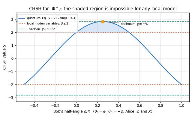
The four Bell states and the circuit that makes them, their correlations and maximally mixed marginals, a full derivation of the local-hidden-variable bound \(\vert S\vert\le2\) and of Tsirelson’s bound \(2\sqrt2\), a simulated shot-by-shot CHSH experiment with error bars, and the fate of the violation under white noise, dephasing and imperfect detectors.

Quantum teleportation — no-cloning, Bell measurement and classical feed-forward

A complete derivation and simulation of quantum teleportation: the no-cloning theorem with proof, the Bell-basis algebra of the protocol, a jit/vmap-compatible mid-circuit measurement with classical feed-forward, uniform outcome statistics and no-signalling, the classical 2/3 benchmark derived from a Haar-averaging identity, teleportation through a noisy Bell pair on the density tensor and via trajectories, and the deferred-measurement circuit.

Entanglement swapping and superdense coding

Two protocols that turn entanglement into a resource: swapping entanglement between particles that never met (with the complete four-qubit algebra, mid-circuit Bell measurement, feed-forward, noisy Werner links and the repeater chain), and sending two classical bits down one qubit, with decoding statistics, the Holevo bound, and the rate and capacity of a noisy shared pair.

GHZ states and decoherence — genuine multipartite entanglement and its fragility

Building N-qubit GHZ states with a CNOT cascade and with a log-depth tree, certifying them through stabilisers, parity oscillations and the fidelity witness, and then watching local dephasing, depolarising and amplitude damping destroy them — analytically, on the density tensor, and with quantum trajectories up to twelve qubits.

Quantum state tomography — linear inversion, least squares and maximum likelihood

How to reconstruct an unknown density matrix from measured click statistics: the Pauli/Bloch linear model and its design matrix, ordinary and weighted least squares with error propagation, the unphysical-estimate problem and its projection fix, the RρR and gradient-based maximum-likelihood estimators, and an accuracy-versus-shots assessment up to four qubits.

Classical shadows — tomography without the \(4^N\) wall

Randomised measurements turned into an unbiased classical description of a quantum state: the measurement channel and its inverse derived for random Pauli bases and for global Clifford ensembles, the single-snapshot estimator and its variance (the shadow norm), median of means, and many observables — correlators, an energy, a fidelity, a reconstructed density matrix — predicted from one data set.