Bright solitons — imaginary-time ground states and real-time dynamics of the nonlinear Schrödinger equation

Marcin Płodzień — Institute of Theoretical Physics, Jagiellonian University in Kraków
ORCID 0000-0002-0835-1644 · github.com/MarcinPlodzien · www

Quantum Many-Body Simulation — Chapter 1 — Computational toolbox

1. Introduction

Quantum mechanics is linear. The superposition principle is one of its axioms: if \(\psi_1\) and \(\psi_2\) solve the Schrödinger equation, so does \(\alpha\psi_1 + \beta\psi_2\). Linearity is what makes the free particle exactly solvable and what lets any state be expanded in energy eigenstates.

This notebook solves an equation that is not linear:

\[ i\,\frac{\partial\psi}{\partial t} \;=\; -\frac{1}{2}\frac{\partial^{2}\psi}{\partial x^{2}} \;-\; g\,\vert\psi\vert^{2}\psi . \tag{1} \]

The last term is cubic in the unknown function: multiplying \(\psi\) by two multiplies it by eight. Superposition is gone, and with it the whole machinery of eigenstates and spectral decomposition. Section 2 explains where such an equation comes from in a theory that is linear by construction. In short, Eq. (1) describes one orbital occupied by \(N\) particles at once, with the other \(N-1\) particles acting on it as an average field, and \(\psi\) is that orbital rather than the wave function of the whole system. It is the Gross-Pitaevskii equation of a Bose-Einstein condensate, introduced independently in [1] and [2], and it is also, with different symbols, the equation for the envelope of a light pulse in a glass fibre.

The physics that motivates it is one specific phenomenon. A free Gaussian wave packet spreads: its width grows as \(\sigma(t) = \sigma_0\sqrt{1+(t/2\sigma_0^2)^2}\) and there is nothing anyone can do about it, because a localised packet necessarily contains a range of momenta and those momenta travel at different speeds. When \(g>0\) in Eq. (1) the particles attract each other, and the attraction can balance the spreading exactly. The result is a bright soliton: a lump of matter that travels for ever at constant velocity, with constant shape and constant width. Two laboratories produced one in 2002 [3], [4] out of a few thousand lithium-7 atoms, and one of them watched it travel \(1.1\,\mathrm{mm}\) without dispersing.

Finding it on a computer needs a new technique. For a linear problem the ground state comes from diagonalising a matrix. That is impossible here: “the Hamiltonian” contains \(\vert\psi\vert^2\), so it depends on the very state we are looking for, and there is no matrix to hand to an eigensolver. The replacement is imaginary-time evolution: run the Schrödinger equation with \(t\) replaced by \(-i\tau\) and every state decays towards the lowest one. Sections 7 and 8 build that idea from the linear case, where everything can be checked against the harmonic oscillator, up to the nonlinear case, where it becomes a gradient flow of the energy.

Road map

• Section 2 — the Hartree argument: \(N\) bosons in one orbital, a contact interaction, and how \(\vert\psi\vert^2\psi\) appears. What is approximated, and where the same equation describes light.
• Section 3 — the 1D Gross-Pitaevskii equation in SI units, the coupling constant \(g_{\rm 1D}\) of a tight waveguide, and the non-dimensionalisation that reduces the problem to the single number \(g\) of Eq. (1). Numbers for the lithium-7 experiments.
• Section 4 — the energy functional, conservation of norm, energy and momentum, and why the chemical potential \(\mu\) differs from the energy per particle.
• Section 5 — the exact soliton, derived: first integral of the stationary equation, the mechanical analogy, the \(\mathrm{sech}\) profile, \(\mu = -g^2/8\), \(E = -g^2/24\); and the Galilean boost.
• Section 6 — the physics: dispersion against attraction, why 1D is safe and 3D collapses, the one-parameter family, \(\mu = dE/dN\), the soliton as a particle, what the mean field hides, integrability, and the limits of the description.
• Sections 7 and 8 — imaginary time: the idea in four layers with a numerical demonstration for each, then the split-step algorithm, its convergence in \(\Delta\tau\), \(N_x\) and \(L\), and its failure modes.
• Section 9 — real time: the stability limit of Runge-Kutta against the unitary split-step method, the stationary soliton, the moving soliton against the spreading linear packet, a non-soliton initial state, convergence and conservation.
• Section 10 — animations and space-time maps.
• Section 11 — summary, an extended workflow checklist, exercises, references.

The notebook assumes the non-dimensionalisation, periodic grid and spectral derivatives of notebook 00a, a free Gaussian wave packet and the potentials, eigenstates and explicit time integrators of notebook 00b, the harmonic oscillator.

What you will learn

Physics

• how a nonlinear equation arises from linear quantum mechanics through a mean-field (Hartree) approximation, and exactly which physics is thrown away in the process;
• the bright soliton: profile, chemical potential, energy, width, and the balance of kinetic dispersion against attractive interaction that produces it;
• why a one-dimensional attractive condensate is stable while a three-dimensional one collapses;
• \(\mu = dE/dN\), self-binding, Galilean invariance, and the soliton as a composite particle;
• what integrability means in practice: a shape that is an attractor of nearby initial conditions.

Numerical methods

• imaginary-time evolution, derived from four independent points of view (spectral decay, diffusion with absorption, the power method, steepest descent on the energy functional);
• the Strang split-step Fourier method in imaginary and in real time, its \(O(\Delta t^2)\) error, and the measured order of the bias it leaves in a converged ground state;
• the stability limit of an explicit Runge-Kutta integrator on a grid, and why an unconditionally stable method changes what is possible;
• convergence monitors for an iterative ground-state solver: energy, chemical potential, residual.

Implementation practice

• one lax.scan body reused for imaginary and real time, compiled once with jax.jit;
• jax.grad for the derivative \(\mu = dE_{\rm tot}/dN\);
• validating a nonlinear solver against a closed-form solution at every stage.

Configuration

Every notebook of this course starts with the same cell. Choose where to run (DEVICE) and the floating-point precision (PRECISION): "double" = float64/complex128 (default, recommended for physics), "single" = float32/complex64 (half the memory, faster on consumer GPUs, but watch the round-off). All code below derives its dtypes from RDTYPE/CDTYPE and its check tolerances from TOL, so nothing else needs to change.

Code

# ==============================================================================
# CONFIGURATION  -- adapt to your hardware, then run the notebook top to bottom
# ==============================================================================
DEVICE    = "auto"     # "auto": use a GPU if JAX finds one, else CPU | "cpu" | "gpu"
PRECISION = "double"   # "double": float64/complex128 | "single": float32/complex64

import os
if DEVICE == "cpu":
    os.environ["JAX_PLATFORMS"] = "cpu"          # must be set BEFORE jax is imported

import string
from functools import partial

import math
import numpy as np
import jax
import jax.numpy as jnp
from jax import lax

# Precision is configurable: "double" = float64/complex128 (default; needed for long time evolutions and
# tight validation), "single" = float32/complex64 (half the memory, faster on consumer GPUs).
jax.config.update("jax_enable_x64", PRECISION == "double")
RDTYPE = jnp.float64 if PRECISION == "double" else jnp.float32       # real dtype
CDTYPE = jnp.complex128 if PRECISION == "double" else jnp.complex64  # complex dtype of all states/operators
TOL = 1e-10 if PRECISION == "double" else 1e-4                       # tolerance for sanity checks (asserts)
_LETTERS = string.ascii_letters  # the 52 einsum index labels a-z, A-Z

import time
import matplotlib.pyplot as plt

if DEVICE == "gpu" and jax.default_backend() == "cpu":
    print("WARNING: DEVICE='gpu' requested but JAX found no GPU -- running on CPU.")
print(f"JAX {jax.__version__} | backend: {jax.default_backend()} | devices: {jax.devices()}")
print(f"precision: {PRECISION} -> real {RDTYPE.__name__}, complex {CDTYPE.__name__}, check tolerance TOL={TOL:g}")

JAX 0.11.0 | backend: cpu | devices: [CpuDevice(id=0)]
precision: double -> real float64, complex complex128, check tolerance TOL=1e-10

2. Where a nonlinear Schrödinger equation comes from

2.1 \(N\) bosons in a single orbital

Take \(N\) identical bosons of mass \(m\) in one dimension, interacting pairwise:

\[ \hat H \;=\; \sum_{j=1}^{N}\left[-\frac{\hbar^2}{2m}\frac{\partial^2}{\partial X_j^2} + V_{\rm ext}(X_j)\right] \;+\; \sum_{j<l} U(X_j - X_l) . \tag{2} \]

The exact ground state of Eq. (2) is a function of \(N\) variables. For \(N = 10^4\) atoms that object cannot be written down, stored, or computed: this is the many-body problem, and the rest of this course is about attacking it with methods whose errors can be controlled. The Hartree approximation, introduced in [5] for many-electron atoms ([6], Chapter 6, and [7] give the version for bosons), cuts through it with one assumption — that every particle occupies the same single-particle orbital \(\varphi(X)\):

\[ \Psi_{\rm Hartree}(X_1,\ldots,X_N) \;=\; \prod_{j=1}^{N}\varphi(X_j), \qquad \int \vert\varphi(X)\vert^2\,dX = 1 . \tag{3} \]

This is the definition of a Bose-Einstein condensate at the mean-field level: one orbital, occupied \(N\) times. (The condensation itself was predicted in [8], building on Bose’s counting of photon states [9].) It is a variational ansatz, so we get the best \(\varphi\) by minimising the energy. Evaluate \(\langle \Psi\vert\hat H\vert\Psi\rangle\) term by term. The one-body part gives \(N\) identical contributions:

\[ \sum_j \left\langle \Psi\left\vert -\frac{\hbar^2}{2m}\partial_{X_j}^2 + V_{\rm ext}(X_j)\right\vert\Psi\right\rangle = N\int \left[\frac{\hbar^2}{2m}\vert\varphi'\vert^2 + V_{\rm ext}\vert\varphi\vert^2\right] dX . \]

The interaction part has \(N(N-1)/2\) identical pairs, and each pair contributes the same double integral because both particles sit in the same orbital:

\[ \sum_{j<l}\left\langle\Psi\vert U(X_j-X_l)\vert\Psi\right\rangle = \frac{N(N-1)}{2}\iint \vert\varphi(X)\vert^2\,U(X-X')\,\vert\varphi(X')\vert^2\, dX\,dX' . \]

Read the last expression: each particle moves in the field produced by the density of all the others. That is what “mean field” means, and it is why the interaction term is quadratic in the density instead of linear.

2.2 The contact interaction

For ultracold atoms the interatomic potential has a range of a few nanometres while the de Broglie wavelength is hundreds of nanometres to micrometres. At such low energies only \(s\)-wave scattering survives, and the true potential can be replaced by a contact pseudopotential that reproduces the same scattering length \(a_s\), introduced in [10] and carried over to the many-body problem in [11] ([6], Chapter 5):

\[ U(X-X') \;=\; g_{\rm 1D}\,\delta(X-X') . \]

The double integral collapses to \(\tfrac12 g_{\rm 1D}\int\vert\varphi\vert^4 dX\). Writing \(\Psi(X) \equiv \sqrt{N}\,\varphi(X)\) so that \(\int\vert\Psi\vert^2 dX = N\) is the particle number, and replacing \(N(N-1)\to N^2\) (an error of relative size \(1/N\), invisible for \(N = 10^3\) and above), the energy becomes

\[ E[\Psi] \;=\; \int\left[\frac{\hbar^{2}}{2m}\left\vert\frac{\partial\Psi}{\partial X}\right\vert^{2} \;+\; V_{\rm ext}(X)\,\vert\Psi\vert^{2} + \frac{g_{\rm 1D}}{2}\vert\Psi\vert^{4}\right] dX . \tag{4} \]

Minimising Eq. (4) at fixed \(\int\vert\Psi\vert^2 = N\) means setting the functional derivative equal to a Lagrange multiplier \(\mu\) times \(\Psi\), \(\delta E/\delta\Psi^{*} = \mu\Psi\):

\[ \left[-\frac{\hbar^{2}}{2m}\frac{\partial^{2}}{\partial X^{2}} + V_{\rm ext}(X) \;+\; g_{\rm 1D}\vert\Psi\vert^{2}\right]\Psi \;=\; \mu\,\Psi , \tag{5} \]

and the corresponding time-dependent equation, whose stationary solutions are \(\Psi\,e^{-i\mu T/\hbar}\), is the Gross-Pitaevskii equation

\[ i\hbar\,\frac{\partial\Psi}{\partial T} \;=\; \left[-\frac{\hbar^{2}}{2m}\frac{\partial^{2}}{\partial X^{2}} + V_{\rm ext}(X) \;+\; g_{\rm 1D}\vert\Psi\vert^{2}\right]\Psi . \tag{6} \]

The factor \(\tfrac12\) in Eq. (4) and its absence in Eq. (6) are consistent: differentiating \(\tfrac12 g\vert\Psi\vert^4 = \tfrac12 g(\Psi^*\Psi)^2\) with respect to \(\Psi^*\) gives \(g\vert\Psi\vert^2\Psi\). Section 4 turns that factor of two into the statement \(\mu \ne E/N\).

2.3 What has been thrown away

The Hartree ansatz (3) is a product state. It therefore contains no correlations whatsoever between particles: the probability of finding one atom at \(X\) and another at \(X'\) factorises exactly. Everything that a real interacting gas does beyond the average — depletion of the condensate, quantum fluctuations, the entanglement between the atoms, atoms outside the condensate mode — is absent by construction. The approximation is good when the gas is dilute (\(n\vert a_s\vert^3 \ll 1\) in three dimensions), almost fully condensed (almost all atoms in the condensate) and large (\(N \gg 1\), so that \(N-1\approx N\)). It is not a controlled expansion in a small parameter that one can push to next order without extra work, and Section 6.5 points at one specific prediction of Eq. (6) that is qualitatively wrong for the true many-body ground state.

Physics insight. The nonlinearity of Eq. (6) does not violate the superposition principle of quantum mechanics. The underlying \(N\)-body Schrödinger equation is perfectly linear; \(\Psi\) is not a probability amplitude for one particle but a classical-field description of an occupied orbital, of the same nature as the classical electromagnetic field that emerges from a coherent state of many photons. The Born rule does not apply to \(\vert\Psi\vert^2\) as a probability density: it is a particle density, in atoms per metre.

2.4 The same equation for light in a fibre

In a glass fibre the refractive index depends weakly on the intensity, \(n = n_0 + n_2 I\) (the optical Kerr effect). Ref. [12] showed that this nonlinearity can balance the group-velocity dispersion of a fibre, and Ref. [13] observed the resulting optical solitons. Writing the electric field of a pulse as a slowly varying envelope \(A(Z,T)\) on a carrier, expanding the propagation constant to second order in frequency, and moving to a frame travelling at the group velocity gives

\[ i\,\frac{\partial A}{\partial Z} \;=\; \frac{\beta_2}{2}\frac{\partial^{2} A}{\partial T_{\rm ret}^{2}} \;-\; \gamma\,\vert A\vert^{2} A , \]

with \(\beta_2\) the group-velocity dispersion, \(T_{\rm ret}\) the retarded time and \(\gamma \propto n_2\). This is Eq. (1) with the roles of space and time exchanged: the propagation distance \(Z\) plays the part of time, and the retarded time \(T_{\rm ret}\) the part of position. For anomalous dispersion (\(\beta_2 < 0\)) the two terms have the relative sign that produces bright solitons, and everything derived in this notebook — the \(\mathrm{sech}\) profile, the width-amplitude relation, the robustness — applies verbatim to optical pulses.

2.5 Attractive interactions and the 2002 experiments

The sign of \(g_{\rm 1D}\) follows the sign of the \(s\)-wave scattering length \(a_s\). For \(a_s > 0\) the interaction is repulsive, the condensate spreads out, and there is no localised state without a trap. For \(a_s < 0\) it is attractive. In three dimensions an attractive condensate is unstable above a critical atom number — it implodes, an event observed in [14] (Section 6.2) and named the “Bosenova” — which is why the experiments confine the gas tightly in two directions and let it move only along the third.

Two groups did exactly that in 2002, both with lithium-7, whose scattering length can be tuned through zero with a magnetic Feshbach resonance ([15]; first observed in a condensate in [16]):

• Ref. [3] released a cloud into a horizontal optical waveguide of radial frequency \(\omega_\perp/2\pi = 710\,\)Hz, at a magnetic field where \(a_s = -0.21\,\)nm, and followed a single soliton over \(1.1\,\)mm with no measurable spreading. The atom number they measure in the soliton is \(6(2)\times10^{3}\); the stability analysis in the same paper puts it between \(4.2\times10^{3}\) and \(5.2\times10^{3}\). The calculations below use \(N = 4.5\times10^{3}\), and Section 6.8 says what the gap between the two numbers means;
• Ref. [4] produced a train of solitons with about \(5000\) atoms per soliton at \(a_s\approx-3a_0 = -0.16\,\)nm. The solitons live in an optical waveguide whose radial confinement is matched to their magnetic trap, \(\omega_\perp/2\pi = 800\,\)Hz, and they oscillate in a shallow axial potential with a period of \(310\,\)ms for many periods.

Section 3.5 puts these numbers into the units of Eq. (1).

3. The 1D Gross-Pitaevskii equation, and its single parameter

3.1 The coupling constant of a waveguide

Equation (6) is one-dimensional, but atoms live in three. The reduction is legitimate when the transverse confinement is so tight that every atom stays in the transverse ground state: with a harmonic transverse trap of frequency \(\omega_\perp\), the transverse oscillator length is

\[ a_\perp \;=\; \sqrt{\frac{\hbar}{m\omega_\perp}} , \]

and the condition is that all the other energies in the problem stay far below \(\hbar\omega_\perp\). Factorising the 3D order parameter as \(\Psi_{\rm 3D}(X,Y,Z) = \Psi(X)\,\chi_0(Y,Z)\) with \(\chi_0\) the transverse ground state and integrating out \(Y,Z\) produces Eq. (6) with an effective one-dimensional coupling constant. Ref. [17] computed it exactly, including the correction from the confinement-induced resonance; to leading order in \(a_s/a_\perp\),

\[ g_{\rm 1D} \;=\; 2\hbar\,\omega_\perp\, a_s . \tag{7} \]

We quote Eq. (7) without deriving it — the derivation is a scattering calculation in a waveguide, not a topic of this course. Its structure is easy to remember: the three-dimensional coupling is \(g_{\rm 3D} = 4\pi\hbar^2 a_s/m\), and dividing by the transverse area \(2\pi a_\perp^2\) occupied by the Gaussian transverse mode gives \(g_{\rm 3D}/(2\pi a_\perp^2) = 2\hbar^2 a_s/(m a_\perp^2) = 2\hbar\omega_\perp a_s\). The full result of [17] carries one extra factor,

\[ g_{\rm 1D} \;=\; \frac{2\hbar\,\omega_\perp\,a_s}{1 - C\,a_s/(\sqrt2\,a_\perp)} , \qquad C = 1.4603\ldots , \]

where the \(\sqrt2\) appears because the transverse length of [17] is built with the reduced mass \(m/2\), \((\hbar/(\tfrac{m}{2}\omega_\perp))^{1/2} = \sqrt2\,a_\perp\). The vanishing denominator is the confinement-induced resonance. Equation (7) is the leading term in \(a_s/a_\perp\), and for the two experiments of Section 2.5 that ratio is \(1.5\times10^{-4}\) and \(1.2\times10^{-4}\): the correction is four orders of magnitude below everything else in this notebook, and we drop it.

3.2 Scaled variables

The equation to be scaled is Eq. (6) without an external potential,

\[ i\hbar\,\frac{\partial\Psi(X,T)}{\partial T} \;=\; -\frac{\hbar^{2}}{2m}\frac{\partial^{2}\Psi}{\partial X^{2}} + g_{\rm 1D}\vert\Psi\vert^{2}\Psi , \qquad \int\vert\Psi\vert^{2}dX = N . \]

As for the free particle, introduce a length \(x_0\) (still free), a time \(t_0\) and an energy \(E_0\), and write

\[ X = x_0\,x , \qquad T = t_0\,t , \qquad \psi(x,t) \;\equiv\; \sqrt{\frac{x_0}{N}}\;\Psi(x_0x,\,t_0t) . \]

The factor \(\sqrt{x_0/N}\) does two jobs at once: \(\sqrt{x_0}\) makes \(\psi\) dimensionless, and \(1/\sqrt{N}\) turns the normalisation \(N\) into \(1\),

\[ \int\vert\psi(x)\vert^{2}dx \;=\; \int \frac{x_0}{N}\vert\Psi\vert^{2}\,\frac{dX}{x_0} \;=\; \frac{1}{N}\int\vert\Psi\vert^{2}dX \;=\; 1 . \]

Substitute \(\Psi = \sqrt{N/x_0}\,\psi\) and use \(\partial_T = t_0^{-1}\partial_t\), \(\partial_X^2 = x_0^{-2}\partial_x^2\):

\[ \frac{i\hbar}{t_0}\sqrt{\frac{N}{x_0}}\,\frac{\partial\psi}{\partial t} \;=\; -\frac{\hbar^{2}}{2mx_0^{2}}\sqrt{\frac{N}{x_0}}\,\frac{\partial^{2}\psi}{\partial x^{2}} \;+\; g_{\rm 1D}\,\frac{N}{x_0}\,\vert\psi\vert^{2}\sqrt{\frac{N}{x_0}}\,\psi . \]

Cancel the common \(\sqrt{N/x_0}\) and divide by \(E_0 = \hbar/t_0\):

\[ i\,\frac{\partial\psi}{\partial t} \;=\; -\frac{\hbar t_0}{2mx_0^{2}}\,\frac{\partial^{2}\psi}{\partial x^{2}} \;+\; \frac{g_{\rm 1D}\,N\,t_0}{\hbar\,x_0}\,\vert\psi\vert^{2}\psi . \]

Choosing

\[ t_0 \;=\; \frac{m x_0^{2}}{\hbar} , \qquad E_0 \;=\; \frac{\hbar}{t_0} \;=\; \frac{\hbar^{2}}{m x_0^{2}} , \]

makes the first coefficient \(1/2\) and turns the second into \(g_{\rm 1D}N m x_0^2/(\hbar^2 x_0) = g_{\rm 1D}Nmx_0/\hbar^2\). Defining

\[ \boxed{\;g \;\equiv\; -\,\frac{N\,g_{\rm 1D}\,m\,x_0}{\hbar^{2}}\;} \qquad\Longrightarrow\qquad i\,\frac{\partial\psi}{\partial t} \;=\; -\frac{1}{2}\frac{\partial^{2}\psi}{\partial x^{2}} \;-\; g\,\vert\psi\vert^{2}\psi , \tag{8} \]

which is Eq. (1). The minus sign in the definition is a convention that makes \(g > 0\) the attractive case (\(g_{\rm 1D} < 0\), i.e. \(a_s < 0\)), which is the one that produces bright solitons. Repulsive interactions are \(g < 0\).

One dimensionless number, \(g\), now carries the mass, the atom number, the scattering length and the transverse confinement. Two experiments with completely different atom numbers and magnetic fields are the same simulation if their \(g\) agree.

3.3 Fixing \(x_0\) so that \(g\) is a pure number

A free particle has no intrinsic length, and one has to be borrowed from the initial state. Equation (8) is different: \(g\) itself depends on \(x_0\), so the choice of \(x_0\) and the value of \(g\) are not independent. There is a distinguished choice. Section 5 will show that the soliton has a width \(2/g\) in units of \(x_0\), i.e. a physical width

\[ \ell \;=\; x_0\cdot\frac{2}{g} \;=\; x_0\,\frac{2\hbar^{2}}{N\vert g_{\rm 1D}\vert m x_0} \;=\; \frac{2\hbar^{2}}{m N \vert g_{\rm 1D}\vert} \;\overset{(7)}{=}\; \frac{\hbar}{m N\omega_\perp\vert a_s\vert} \;=\; \frac{a_\perp^{2}}{N\vert a_s\vert} , \tag{9} \]

which does not contain \(x_0\) at all, as it must not. Setting \(x_0 = \ell\) then forces

\[ \frac{2}{g} = 1 \qquad\Longrightarrow\qquad g = 2 . \]

Every bright soliton described by Eq. (6) is the same solution of Eq. (8) with \(g = 2\); the only thing that changes from one experiment to another is what one metre and one second mean. We will use \(g = 2\) throughout, and vary \(g\) only where the point is the dependence on \(g\) itself.

3.4 The unit table

quantity	unit	value
length	\(x_0 = \ell = a_\perp^{2}/(N\vert a_s\vert)\)	the soliton width
time	\(t_0 = m x_0^{2}/\hbar\)	derived
energy	\(E_0 = \hbar^{2}/(m x_0^{2})\)	derived
velocity	\(v_0 = x_0/t_0 = \hbar/(m x_0)\)	derived
density	\(1/x_0\)	\(\vert\psi\vert^{2}\) integrates to \(1\)

A physical energy per particle is \(E_0\) times the dimensionless energy; the total energy of the cloud is \(N E_0\) times it, because we normalised \(\psi\) to one rather than to \(N\). Section 6.3 uses that distinction.

3.5 Numbers for the lithium-7 experiments

The cell below is arithmetic only. It takes the published parameters of the two 2002 experiments, builds \(a_\perp\), \(g_{\rm 1D}\), the soliton width \(\ell\) of Eq. (9) and the unit system, and checks that the resulting \(g\) really is \(2\). It also prints the dimensionless combination

\[ \kappa \;\equiv\; \frac{N\vert a_s\vert}{a_\perp} \;=\; \frac{a_\perp}{\ell} , \]

which Section 6.8 identifies as the parameter that decides whether the quasi-one-dimensional description is valid at all.

Code

# ==============================================================================
# EXTRA IMPORTS  -- everything else comes from the Configuration cell above
# ==============================================================================
import base64                                   # to inline the animated GIFs in the notebook output
import tempfile                                 # a scratch file for each GIF (deleted immediately)

from matplotlib.animation import FuncAnimation, PillowWriter   # GIF writing
from IPython.display import display                            # embed the GIF in the notebook output

# colour-blind-friendly palette, used consistently in every figure of this notebook
C_NUM, C_ANA, C_THIRD, C_GREY = "#0072B2", "#D55E00", "#009E73", "0.45"

print("extra imports OK")

extra imports OK

Code

# ==============================================================================
# STEP 0: the unit system of a real bright soliton  (pure bookkeeping, no physics happens here)
#   a_perp = sqrt(hbar / (m omega_perp))          transverse oscillator length
#   g_1D   = 2 hbar omega_perp a_s                Ref. [17], leading order
#   ell    = a_perp^2 / (N |a_s|)                 soliton width, Eq. (9)  -> we set x_0 = ell
#   t_0    = m x_0^2 / hbar,  E_0 = hbar / t_0,  v_0 = x_0 / t_0
# ==============================================================================
HBAR_SI = 1.054571817e-34          # reduced Planck constant                [J s]
AMU     = 1.66053906660e-27        # atomic mass unit                       [kg]
M_LI7   = 7.0160034366 * AMU       # mass of a lithium-7 atom               [kg]


def soliton_units(N, a_s_m, nu_perp_hz, mass_kg=M_LI7):
    """Everything about a quasi-1D bright soliton, from the three numbers an experimentalist quotes.

    MATH
        a_perp = sqrt(hbar / (m * 2 pi nu_perp))
        g_1D   = 2 hbar (2 pi nu_perp) a_s                      [J m]     (a_s < 0 for attraction)
        ell    = a_perp^2 / (N |a_s|)                           [m]       the soliton width
        x_0    = ell,  t_0 = m x_0^2 / hbar,  E_0 = hbar / t_0,  v_0 = x_0 / t_0
        g      = -N g_1D m x_0 / hbar^2                         [-]       must come out as 2
        kappa  = N |a_s| / a_perp = a_perp / ell                [-]       quasi-1D / collapse parameter
    Returns a dict of SI floats plus the two dimensionless numbers.
    """
    omega_perp = 2.0 * np.pi * nu_perp_hz
    a_perp = np.sqrt(HBAR_SI / (mass_kg * omega_perp))
    g_1d = 2.0 * HBAR_SI * omega_perp * a_s_m                   # negative when a_s is negative
    ell = a_perp ** 2 / (N * abs(a_s_m))
    x0 = ell
    t0 = mass_kg * x0 ** 2 / HBAR_SI
    E0 = HBAR_SI / t0
    return {"a_perp": a_perp, "g_1d": g_1d, "ell": ell, "t0": t0, "E0": E0, "v0": x0 / t0,
            "g": -N * g_1d * mass_kg * x0 / HBAR_SI ** 2,
            "kappa": N * abs(a_s_m) / a_perp}


experiments = [("Ref. [3]", 4500, -0.21e-9, 710.0),
               ("Ref. [4]", 5000, -0.16e-9, 800.0)]

print(f"{'experiment':24s} {'a_perp[um]':>10s} {'ell[um]':>9s} {'t_0[ms]':>9s} "
      f"{'E_0/h[Hz]':>10s} {'v_0[mm/s]':>10s} {'g':>7s} {'kappa':>7s}")
for name, N_at, a_s, nu in experiments:
    u = soliton_units(N_at, a_s, nu)
    print(f"{name:24s} {u['a_perp'] * 1e6:10.3f} {u['ell'] * 1e6:9.3f} {u['t0'] * 1e3:9.4f} "
          f"{u['E0'] / (2 * np.pi * HBAR_SI):10.1f} {u['v0'] * 1e3:10.3f} {u['g']:7.4f} {u['kappa']:7.3f}")

# the choice x_0 = ell must give g = 2 exactly -- this is a check of the algebra of Section 3.3
for name, N_at, a_s, nu in experiments:
    assert abs(soliton_units(N_at, a_s, nu)["g"] - 2.0) < 1e4 * TOL, "x_0 = ell must force g = 2"
print("\ncheckpoint: x_0 = ell gives g = 2 for both experiments (to round-off)")

experiment               a_perp[um]   ell[um]   t_0[ms]  E_0/h[Hz]  v_0[mm/s]       g   kappa
Ref. [3]                      1.424     2.147    0.5093      312.5      4.216  2.0000   0.663
Ref. [4]                      1.342     2.251    0.5598      284.3      4.021  2.0000   0.596

checkpoint: x_0 = ell gives g = 2 for both experiments (to round-off)

Both experiments end up with a soliton about \(2.2\,\mu\mathrm{m}\) wide, a time unit of about half a millisecond and an energy unit of \(313\) and \(284\,\mathrm{Hz}\) — the scales a cold-atom laboratory works with. The velocity unit is \(4\,\mathrm{mm/s}\), so the \(1.1\,\mathrm{mm}\) of free propagation reported in [3] is \(1.1\,\mathrm{mm}/2.15\,\mu\mathrm{m} = 512\) length units, which at one unit of velocity would take \(512\) time units, i.e. \(0.26\,\mathrm{s}\). The last column is the one to watch: \(\kappa = a_\perp/\ell\) is \(0.663\) and \(0.596\), so the soliton is only \(1.5\) to \(1.7\) times wider than the transverse ground state. These experiments are quasi-1D by a factor of order two, and Section 6.8 explains why they cannot simply increase \(N\) to do better. Because \(\kappa\propto N\), the last column is also the least certain number in the table: Section 6.8 and the cell there make that explicit.

The check at the end is the first of many: the algebra that led from Eq. (6) to Eq. (8) predicts \(g=2\) when \(x_0\) is the soliton width, and the arithmetic confirms it.

4. Conserved quantities

Equation (8) has no potential and no explicit time dependence, so we expect conservation laws. They are the only independent checks available for a nonlinear problem, so we derive them rather than quote them.

4.1 The energy functional

Rewriting Eq. (4) in the dimensionless variables of Section 3.2, with the total energy measured in units of \(NE_0\) (energy per particle in units of \(E_0\)),

\[ E[\psi] \;=\; \int\left[\frac{1}{2}\left\vert\frac{\partial\psi}{\partial x}\right\vert^{2} \;-\; \frac{g}{2}\vert\psi\vert^{4}\right] dx \;\equiv\; E_{\rm kin} + E_{\rm int} . \tag{10} \]

Its functional derivative with respect to \(\psi^{*}\) is, integrating the first term by parts on the ring,

\[ \frac{\delta E}{\delta\psi^{*}} \;=\; -\frac{1}{2}\frac{\partial^{2}\psi}{\partial x^{2}} \;-\; g\vert\psi\vert^{2}\psi \;\equiv\; \hat H_{\rm GP}[\psi]\,\psi , \tag{11} \]

so Eq. (8) is exactly \(i\,\partial_t\psi = \delta E/\delta\psi^{*}\). The object \(\hat H_{\rm GP}[\psi]\) is written with a hat because it acts like an operator, but the square bracket is essential: it depends on the state it acts on. It is not a matrix, it has no eigenbasis, and nothing from the linear eigenvalue problem applies to it.

4.2 Norm

Multiply Eq. (8) by \(\psi^{*}\), subtract the complex conjugate, and divide by \(i\):

\[ \frac{\partial\vert\psi\vert^{2}}{\partial t} \;=\; \frac{i}{2}\left(\psi^{*}\psi'' - \psi\,\psi^{*\prime\prime}\right) \;+\; i\,g\left(\vert\psi\vert^{2}\psi^{*}\psi - \vert\psi\vert^{2}\psi\psi^{*}\right) . \]

The interaction term cancels identically — it is real and multiplies \(\vert\psi\vert^2\) — which is the whole reason the nonlinearity does not destroy probability conservation. The first term is a total derivative,

\[ \frac{\partial\vert\psi\vert^{2}}{\partial t} + \frac{\partial j}{\partial x} = 0 , \qquad j \;=\; \mathrm{Im}\left(\psi^{*}\frac{\partial\psi}{\partial x}\right) , \tag{12} \]

the ordinary continuity equation. On a ring the integral of \(\partial_x j\) vanishes, so \(\int\vert\psi\vert^{2}dx\) is conserved.

4.3 Energy

Because \(E\) is real, \(\delta E/\delta\psi = (\delta E/\delta\psi^{*})^{*}\), and the chain rule gives

\[ \frac{dE}{dt} \;=\; \int\left(\frac{\delta E}{\delta\psi}\frac{\partial\psi}{\partial t} + \frac{\delta E}{\delta\psi^{*}}\frac{\partial\psi^{*}}{\partial t}\right) dx \;=\; 2\,\mathrm{Re}\int \left(\hat H_{\rm GP}\psi\right)\frac{\partial\psi^{*}}{\partial t}\,dx . \]

Equation (8) says \(\partial_t\psi = -i\hat H_{\rm GP}\psi\), hence \(\partial_t\psi^{*} = +i(\hat H_{\rm GP}\psi)^{*}\), and

\[ \frac{dE}{dt} \;=\; 2\,\mathrm{Re}\left[\,i\int\left\vert \hat H_{\rm GP}\psi\right\vert^{2}dx\right] \;=\; 0 , \tag{13} \]

because the integral is real and non-negative and \(i\) times a real number is purely imaginary. The same three lines, with \(-i\) replaced by \(-1\), will give the monotonic decrease of the energy in imaginary time (Section 7.5).

4.4 Momentum

The expectation value \(\langle p\rangle = \int\psi^{*}(-i\partial_x)\psi\,dx = \int j\,dx\) is conserved for the same reason as for the free particle: Eq. (8) is invariant under translations. Ehrenfest’s relation [18] also survives unchanged,

\[ \frac{d\langle x\rangle}{dt} \;=\; \langle p\rangle . \tag{14} \]

Both statements follow from Eq. (12), in which the interaction has already cancelled. For Eq. (14), multiply Eq. (12) by \(x\) and integrate by parts once: \(d\langle x\rangle/dt = \int x\,\partial_t\vert\psi\vert^{2}dx = -\int x\,\partial_x j\,dx = \int j\,dx = \langle p\rangle\), the boundary term vanishing on the ring. For \(\langle p\rangle\) itself the same manipulation on Eq. (8) gives a local conservation law \(\partial_t j + \partial_x\Pi = 0\) with a momentum flux \(\Pi\) whose interaction part is \(-\tfrac{g}{2}\vert\psi\vert^{4}\); since \(\Pi\) is a single-valued function on the ring, \(d\langle p\rangle/dt = -\int\partial_x\Pi\,dx = 0\). The interaction can only move momentum from one place to another, never create it — which is what “invariant under translations” means. Section 6.4 makes this the statement that a soliton moves like a free particle.

4.5 Chemical potential and energy per particle

A stationary state of Eq. (8) is \(\psi(x,t) = \phi(x)e^{-i\mu t}\) with \(\phi\) time-independent. Substituting, \(i\partial_t\psi = \mu\phi e^{-i\mu t}\), so

\[ \hat H_{\rm GP}[\phi]\,\phi \;=\; -\frac{1}{2}\phi'' - g\vert\phi\vert^{2}\phi \;=\; \mu\,\phi , \tag{15} \]

which is Eq. (5) non-dimensionalised. Multiplying by \(\phi^{*}\) and integrating over a normalised \(\phi\),

\[ \mu \;=\; \int\left[\frac{1}{2}\vert\phi'\vert^{2} - g\vert\phi\vert^{4}\right]dx \;=\; E_{\rm kin} + 2E_{\rm int} , \tag{16} \]

whereas the energy per particle is \(E = E_{\rm kin} + E_{\rm int}\) by Eq. (10). The two differ by exactly \(E_{\rm int}\): the interaction energy is shared between pairs, so counting it once per particle double-counts it. For the soliton \(E_{\rm int}<0\) and therefore \(\mu < E\). Section 6.3 gives the identity behind this, \(\mu = dE_{\rm tot}/dN\), and verifies it numerically.

Common pitfall. In a linear problem \(\mu\) and \(E\) coincide and nobody distinguishes them. Reporting a Gross-Pitaevskii “energy” without saying which of the two it is, is one of the standard ways of being wrong; for the soliton of Section 5 the two differ by a factor of three.

5. The exact bright soliton

5.1 The stationary equation as a mechanics problem

Look for a stationary state with a real profile, \(\psi = \phi(x)e^{-i\mu t}\) with \(\phi\) real. (A complex \(\phi\) would carry a current; on an infinite line with \(\phi\to0\) at both ends there is nowhere for a current to go, so nothing is lost.) Equation (15) becomes an ordinary differential equation,

\[ \phi'' \;=\; -2g\,\phi^{3} - 2\mu\,\phi . \tag{17} \]

This is Newton’s second law for a unit-mass particle whose “position” is \(\phi\) and whose “time” is \(x\), moving in the potential \(U(\phi)\) defined by \(\phi'' = -dU/d\phi\):

\[ \frac{dU}{d\phi} = 2g\phi^{3} + 2\mu\phi \qquad\Longrightarrow\qquad U(\phi) \;=\; \frac{g}{2}\phi^{4} + \mu\,\phi^{2} . \]

Mechanics then supplies a first integral for free — the conserved “energy” of the analogue particle,

\[ \frac{1}{2}\left(\phi'\right)^{2} + U(\phi) \;=\; C \qquad\text{(independent of }x\text{)} . \tag{18} \]

To verify Eq. (18), differentiate it with respect to \(x\): \(\phi'\phi'' + U'(\phi)\phi' = \phi'(\phi'' + U') = 0\) by Eq. (17).

A bright soliton is a localised solution: \(\phi\to0\) and \(\phi'\to0\) as \(\vert x\vert\to\infty\). Evaluating Eq. (18) in that limit fixes \(C = 0\), so

\[ \left(\phi'\right)^{2} \;=\; -g\phi^{4} - 2\mu\phi^{2} . \tag{19} \]

The right-hand side must be non-negative near \(\phi = 0\), where the \(\phi^2\) term dominates; therefore \(\mu < 0\). Write \(\mu = -\kappa^{2}/2\) with \(\kappa > 0\), so that

\[ \left(\phi'\right)^{2} \;=\; \kappa^{2}\phi^{2} - g\phi^{4} \;=\; \phi^{2}\left(\kappa^{2} - g\phi^{2}\right) . \tag{20} \]

For \(g < 0\) (repulsion) the bracket never vanishes, \(\phi\) grows without bound, and there is no localised solution at all. For \(g > 0\) the analogue particle starts at \(\phi = 0\) with zero velocity in the infinite past, is pushed out to the turning point \(\phi_{\max} = \kappa/\sqrt{g}\) where \(\phi' = 0\), and returns — one excursion, which is the soliton.

5.2 Integrating to the profile

Take the branch with \(\phi' < 0\) (the decaying side, \(x > x_c\)) and separate variables:

\[ \frac{d\phi}{\phi\sqrt{\kappa^{2}-g\phi^{2}}} \;=\; -\,dx . \]

Substitute \(\phi = (\kappa/\sqrt{g})\,s\), so \(d\phi = (\kappa/\sqrt{g})\,ds\) and \(\sqrt{\kappa^2 - g\phi^2} = \kappa\sqrt{1-s^{2}}\):

\[ \frac{(\kappa/\sqrt g)\,ds}{(\kappa/\sqrt g)\,s\cdot\kappa\sqrt{1-s^{2}}} \;=\; \frac{1}{\kappa}\,\frac{ds}{s\sqrt{1-s^{2}}} \;=\; -\,dx . \]

The remaining integral is elementary,

\[ \int\frac{ds}{s\sqrt{1-s^{2}}} \;=\; -\,\mathrm{arcsech}(s) \;=\; -\ln\!\left(\frac{1+\sqrt{1-s^{2}}}{s}\right) , \]

as one checks by differentiating: with \(s = \mathrm{sech}\,\theta\) one has \(ds = -\mathrm{sech}\,\theta\tanh\theta\,d\theta\) and \(\sqrt{1-s^2} = \tanh\theta\), so the integrand becomes \(-d\theta\). Therefore

\[ -\frac{1}{\kappa}\,\mathrm{arcsech}(s) \;=\; -x + \text{const} \qquad\Longrightarrow\qquad s \;=\; \mathrm{sech}\!\left[\kappa(x-x_c)\right] , \]

and, undoing the substitution,

\[ \boxed{\;\phi(x) \;=\; \frac{\kappa}{\sqrt{g}}\;\mathrm{sech}\!\left[\kappa\,(x-x_c)\right]\;} \tag{21} \]

with two constants of integration: the centre \(x_c\) (translation invariance) and \(\kappa\), which Eq. (20) ties to \(\mu = -\kappa^{2}/2\).

5.3 Fixing \(\kappa\) by the normalisation

Using \(\int_{-\infty}^{\infty}\mathrm{sech}^{2}(\kappa u)\,du = 2/\kappa\),

\[ \int\phi^{2}dx \;=\; \frac{\kappa^{2}}{g}\cdot\frac{2}{\kappa} \;=\; \frac{2\kappa}{g} \;\overset{!}{=}\; 1 \qquad\Longrightarrow\qquad \kappa = \frac{g}{2} . \]

Substituting back:

\[ \phi(x) \;=\; \frac{\sqrt g}{2}\;\mathrm{sech}\!\left[\frac{g}{2}(x-x_c)\right] , \qquad \mu \;=\; -\frac{g^{2}}{8} . \tag{22} \]

The energy follows from Eq. (10) with \(\int\mathrm{sech}^{4}(\kappa u)du = 4/(3\kappa)\) and \(\int\mathrm{sech}^{2}\tanh^{2}(\kappa u)\,du = 2/(3\kappa)\) (the second follows from the first and \(\tanh^2 = 1-\mathrm{sech}^2\)):

\[ \begin{aligned} E_{\rm kin} &= \frac{1}{2}\int\left(\phi'\right)^{2}dx = \frac{1}{2}\,\frac{\kappa^{2}}{g}\,\kappa^{2}\int\mathrm{sech}^{2}\tanh^{2} = \frac{1}{2}\,\frac{\kappa^{4}}{g}\,\frac{2}{3\kappa} = \frac{\kappa^{3}}{3g} = \frac{g^{2}}{24} , \\[4pt] E_{\rm int} &= -\frac{g}{2}\int\phi^{4}dx = -\frac{g}{2}\,\frac{\kappa^{4}}{g^{2}}\,\frac{4}{3\kappa} = -\frac{2\kappa^{3}}{3g} = -\frac{g^{2}}{12} , \end{aligned} \]

so that

\[ E \;=\; E_{\rm kin} + E_{\rm int} \;=\; -\frac{g^{2}}{24} , \qquad \mu \;=\; E_{\rm kin} + 2E_{\rm int} \;=\; \frac{g^{2}}{24} - \frac{g^{2}}{6} = -\frac{g^{2}}{8} , \tag{23} \]

the second line reproducing Eq. (22) and confirming Eq. (16). The relation \(E_{\rm int} = -2E_{\rm kin}\) is exact: it is the one-dimensional virial theorem for a cubic nonlinearity, and Exercise 3 asks for its derivation.

Two more numbers we will measure. The width of the density \(\vert\phi\vert^2\), defined as its standard deviation, uses \(\int u^{2}\mathrm{sech}^{2}(\kappa u)du = \pi^{2}/(6\kappa^{3})\):

\[ \mathrm{Var}(x) \;=\; \frac{\kappa^{2}}{g}\cdot\frac{\pi^{2}}{6\kappa^{3}} \;=\; \frac{\pi^{2}}{3g^{2}} , \qquad \sigma \;=\; \frac{\pi}{\sqrt3\,g} \;\approx\; \frac{1.8138}{g} , \tag{24} \]

and the peak density is \(\phi(x_c)^{2} = g/4\). The decay length of the amplitude is \(2/g\) — the number we used in Section 3.3 to fix \(x_0\).

5.4 A soliton of arbitrary norm

Nothing in Sections 5.1-5.2 used the normalisation; Eq. (21) solves Eq. (15) for any \(\kappa\). Repeating Section 5.3 with \(\int\phi^{2}dx = n\) gives \(\kappa = ng/2\), so

\[ \phi_n(x) = \frac{n\sqrt g}{2}\,\mathrm{sech}\!\left[\frac{ng}{2}(x-x_c)\right] , \qquad \mu_n = -\frac{(ng)^{2}}{8} . \tag{25} \]

Since \(g\propto N\) (Section 3.2), the combination \(ng\) is proportional to the number of atoms in that soliton. Equation (25) therefore says: twice as many atoms, half the width, twice the peak amplitude, four times the binding. Section 6.3 develops this.

5.5 The grid, and the functions that encode Sections 4 and 5

The discretisation is the one of notebook 00a, a free Gaussian wave packet: a periodic ring of circumference \(L\) with \(N_x\) points, the FFT wave numbers from np.fft.fftfreq, spectral derivatives, and Riemann sums for the integrals. One change: the grid is centred, \(x_j \in [-L/2, L/2)\), so that a soliton at \(x_c = 0\) sits in the middle of the array rather than on the seam.

The ring is not the infinite line, so the \(\mathrm{sech}\) of Eq. (22) is not an exact solution on it: the periodic images add a correction of relative size \(e^{-gL/4}\) (the amplitude of the tail at the far side of the ring). For \(g=2\) and \(L=60\) that is \(e^{-30} \approx 10^{-13}\), which sets the floor of every check below.

Below: make_grid, the exact solution soliton_exact including the Galilean boost of Section 5.6, gp_hamiltonian for \(\hat H_{\rm GP}\psi\), and the three energies.

Code

# ==============================================================================
# STEP 1: grid, exact solution, and the GP functionals
# ==============================================================================
def make_grid(L, N_x):
    """Centred periodic grid on [-L/2, L/2) and the matching FFT wave numbers.

    MATH
        x_j = (j - N_x/2) dx,  j = 0..N_x-1,  dx = L / N_x
        k_n = 2 pi n / L in np.fft.fft order (n = 0,1,..,N_x/2-1,-N_x/2,..,-1)
    """
    dx = L / N_x
    x = (np.arange(N_x) - N_x // 2) * dx
    k = 2.0 * np.pi * np.fft.fftfreq(N_x, d=dx)
    return x, k, dx


def soliton_exact(x, t=0.0, g=2.0, x_c=0.0, k_0=0.0, n=1.0):
    """The bright soliton of the NLS equation, boosted to velocity k_0 -- Eqs. (22), (25), (27).

    MATH
        kappa = n g / 2,   mu = -kappa^2 / 2,   amplitude = kappa / sqrt(g)
        psi(x,t) = (kappa/sqrt(g)) sech[kappa (x - x_c - k_0 t)]
                   * exp( i k_0 x - i (k_0^2/2 + mu) t )
        integral |psi|^2 dx = n   (n = 1 unless stated otherwise)
    IMPLEMENTATION
        The sech is evaluated as 1/cosh; for |argument| > 710 cosh overflows, so the argument is clipped.
        On a ring this function is exact only up to the periodic-image correction ~ exp(-kappa L / 2).
    """
    kappa = n * g / 2.0
    mu = -0.5 * kappa ** 2
    u = np.clip(kappa * (x - x_c - k_0 * t), -700.0, 700.0)
    envelope = (kappa / np.sqrt(g)) / np.cosh(u)
    phase = np.exp(1j * (k_0 * x - (0.5 * k_0 ** 2 + mu) * t))
    return (envelope * phase).astype(CDTYPE)


def d_dx(psi, k):
    """Spectral first derivative:  psi'(x) = IFFT[ i k FFT[psi] ]  (exact for band-limited periodic psi)."""
    return np.fft.ifft(1j * k * np.fft.fft(psi))


def d2_dx2(psi, k):
    """Spectral second derivative:  psi''(x) = IFFT[ -k^2 FFT[psi] ]."""
    return np.fft.ifft(-(k ** 2) * np.fft.fft(psi))


def gp_hamiltonian(psi, k, g, V=0.0):
    """Apply the Gross-Pitaevskii operator -- Eq. (11).

    MATH
        H_GP[psi] psi = -(1/2) psi'' - g |psi|^2 psi + V psi
    NOTE
        This is NOT a linear operator: it depends on psi through |psi|^2.
    """
    return -0.5 * d2_dx2(psi, k) - g * np.abs(psi) ** 2 * psi + V * psi


def gp_energy(psi, k, dx, g, V=0.0, parts=False):
    """Energy per particle in units of E_0 -- Eq. (10) plus an optional trap term.

    MATH
        E = dx sum_j [ (1/2)|psi'_j|^2 - (g/2)|psi_j|^4 + V_j |psi_j|^2 ]
    IMPLEMENTATION
        The derivative is spectral, so on a smooth periodic state E is accurate to round-off.
        parts=True returns (E_kin, E_int, E_pot) separately, which Eq. (16) needs.
    """
    e_kin = float(dx * np.sum(0.5 * np.abs(d_dx(psi, k)) ** 2).real)
    e_int = float(dx * np.sum(-0.5 * g * np.abs(psi) ** 4))
    e_pot = float(dx * np.sum(V * np.abs(psi) ** 2))
    return (e_kin, e_int, e_pot) if parts else e_kin + e_int + e_pot


def gp_chemical_potential(psi, k, dx, g, V=0.0):
    """mu = <psi| H_GP[psi] |psi> for a normalised psi -- Eq. (16)."""
    return float(dx * np.sum(np.conj(psi) * gp_hamiltonian(psi, k, g, V)).real)


def gp_residual(psi, k, dx, g, V=0.0):
    """L2 norm of  H_GP[psi] psi - mu psi  with mu = <H_GP>: zero exactly on a stationary state."""
    mu = gp_chemical_potential(psi, k, dx, g, V)
    r = gp_hamiltonian(psi, k, g, V) - mu * psi
    return float(np.sqrt(dx * np.sum(np.abs(r) ** 2)))


def grid_norm(psi, dx):
    """Norm squared:  dx sum_j |psi_j|^2  (should be 1 throughout this notebook)."""
    return float(dx * np.sum(np.abs(psi) ** 2))


def normalise(psi, dx):
    """Rescale so that dx sum |psi|^2 = 1."""
    return psi / np.sqrt(grid_norm(psi, dx))


print("STEP 1 functions defined:", ", ".join(
    ["make_grid", "soliton_exact", "gp_hamiltonian", "gp_energy", "gp_chemical_potential", "gp_residual"]))

STEP 1 functions defined: make_grid, soliton_exact, gp_hamiltonian, gp_energy, gp_chemical_potential, gp_residual

5.6 Measuring position, width and momentum on a ring

Three observables, the standard grid estimators adapted to the centred grid. The mean position uses the circular mean — map each grid point to the unit circle, average with weight \(\vert\psi_j\vert^2\Delta x\), read off the angle — so that it keeps working when the soliton crosses the seam at \(\pm L/2\); the variance uses the wrapped distance to that mean; the mean momentum is computed in Fourier space, where \(\hat p\) is diagonal.

Code

# ==============================================================================
# STEP 2: observables on a ring  (as in 'A free Gaussian wave packet on a ring')
# ==============================================================================
def mean_position(psi, x, dx, L):
    """Circular mean of |psi|^2, returned in (-L/2, L/2].

    MATH
        z = dx sum_j |psi_j|^2 exp(2 pi i x_j / L);   <x> = (L / 2 pi) arg(z)
    """
    w = np.abs(psi) ** 2 * dx
    z = np.sum(w * np.exp(2j * np.pi * x / L))
    return float(np.angle(z)) * L / (2.0 * np.pi)


def position_variance(psi, x, dx, L):
    """Var(x) measured with the shortest signed distance on the ring.

    MATH
        d_j = ((x_j - <x> + L/2) mod L) - L/2
        Var = sum_j d_j^2 |psi_j|^2 dx / sum_j |psi_j|^2 dx
    CAVEAT
        Meaningful only while the state is much narrower than the ring (sigma << L/4).
    """
    xbar = mean_position(psi, x, dx, L)
    d = (x - xbar + 0.5 * L) % L - 0.5 * L
    w = np.abs(psi) ** 2 * dx
    return float(np.sum(d ** 2 * w) / np.sum(w))


def mean_momentum(psi, k):
    """Momentum PER PARTICLE, evaluated in Fourier space.

    MATH
        <p>/N = sum_n k_n |psi_hat_n|^2 / sum_n |psi_hat_n|^2
    NOTE
        The weights are normalised, so this equals <psi| -i d/dx |psi> only for a state of unit norm
        (the case throughout this notebook); multiply by the norm to obtain the total momentum.
    """
    weights = np.abs(np.fft.fft(psi)) ** 2
    return float(np.sum(k * weights) / np.sum(weights))


print("STEP 2 observables defined: mean_position, position_variance, mean_momentum")

STEP 2 observables defined: mean_position, position_variance, mean_momentum

5.7 Numerical check of the exact solution

Everything derived in Sections 5.1-5.3 is now checked numerically: the norm, the residual \(\Vert \hat H_{\rm GP}\phi - \mu\phi\Vert\) with the predicted \(\mu = -g^2/8\), the energies \(E_{\rm kin} = g^2/24\), \(E_{\rm int} = -g^2/12\), \(E = -g^2/24\), the identity \(\mu = E_{\rm kin}+2E_{\rm int}\), the width \(\pi/(\sqrt3 g)\) and the peak density \(g/4\). Nothing here is fitted; every number on the right of each line came out of the algebra above.

Code

# ==============================================================================
# PARAMETERS of the main experiment  (change them and re-run the whole notebook)
# ==============================================================================
G      = 2.0       # dimensionless coupling; g = 2 <=> x_0 is the soliton width (Section 3.3)
L      = 60.0      # circumference of the ring          [x_0]
N_X    = 512       # number of grid points              [-]

x, k, dx = make_grid(L, N_X)

print(f"grid    : L = {L}, N_x = {N_X}, dx = {dx:.6f}, Nyquist k = {np.pi / dx:.3f}")
print(f"soliton : g = {G}, width 2/g = {2 / G:.3f}, sigma = pi/(sqrt3 g) = {np.pi / (np.sqrt(3) * G):.6f}, "
      f"peak density g/4 = {G / 4:.3f}")
print(f"ring    : periodic-image correction ~ exp(-g L / 4) = {np.exp(-G * L / 4):.2e}  -> the error floor below")

grid    : L = 60.0, N_x = 512, dx = 0.117188, Nyquist k = 26.808
soliton : g = 2.0, width 2/g = 1.000, sigma = pi/(sqrt3 g) = 0.906900, peak density g/4 = 0.500
ring    : periodic-image correction ~ exp(-g L / 4) = 9.36e-14  -> the error floor below

Code

# ==============================================================================
# CHECKPOINT 1: the sech profile solves the stationary GP equation
# ==============================================================================
phi = soliton_exact(x, t=0.0, g=G)

mu_exact = -G ** 2 / 8.0
e_kin, e_int, _ = gp_energy(phi, k, dx, G, parts=True)
e_tot = e_kin + e_int
mu_num = gp_chemical_potential(phi, k, dx, G)
res = np.sqrt(dx * np.sum(np.abs(gp_hamiltonian(phi, k, G) - mu_exact * phi) ** 2))
var_num = position_variance(phi, x, dx, L)

rows = [("norm",                grid_norm(phi, dx),        1.0),
        ("mu = <H_GP>",         mu_num,                    -G ** 2 / 8),
        ("E_kin",               e_kin,                     G ** 2 / 24),
        ("E_int",               e_int,                     -G ** 2 / 12),
        ("E = E_kin + E_int",   e_tot,                     -G ** 2 / 24),
        ("E_kin + 2 E_int",     e_kin + 2 * e_int,         -G ** 2 / 8),
        ("Var(x)",              var_num,                   np.pi ** 2 / (3 * G ** 2)),
        ("sigma",               np.sqrt(var_num),          np.pi / (np.sqrt(3) * G)),
        ("peak density",        float(np.max(np.abs(phi) ** 2)), G / 4),
        ("<p>",                 mean_momentum(phi, k),     0.0)]

print(f"{'quantity':22s} {'numerical':>18s} {'analytic':>18s} {'difference':>12s}")
for name, num, ana in rows:
    print(f"{name:22s} {num:18.12f} {ana:18.12f} {abs(num - ana):12.2e}")
    assert abs(num - ana) < 1e-9, f"{name} disagrees with the analytic value"

print(f"\nresidual || H_GP phi - mu phi ||   = {res:.3e}   (floor set by the periodic images, see above)")
assert res < 1e-9, "the sech must solve the stationary equation on this grid"
print("CHECKPOINT 1 passed: Eqs. (22)-(24) verified on the grid.")

quantity                        numerical           analytic   difference
norm                       1.000000000000     1.000000000000     2.22e-16
mu = <H_GP>               -0.500000000000    -0.500000000000     1.11e-16
E_kin                      0.166666666667     0.166666666667     0.00e+00
E_int                     -0.333333333333    -0.333333333333     0.00e+00
E = E_kin + E_int         -0.166666666667    -0.166666666667     0.00e+00
E_kin + 2 E_int           -0.500000000000    -0.500000000000     0.00e+00
Var(x)                     0.822467033424     0.822467033424     1.11e-16
sigma                      0.906899682117     0.906899682117     1.11e-16
peak density               0.500000000000     0.500000000000     1.11e-16
<p>                       -0.000000000000     0.000000000000     2.60e-17

residual || H_GP phi - mu phi ||   = 5.567e-13   (floor set by the periodic images, see above)
CHECKPOINT 1 passed: Eqs. (22)-(24) verified on the grid.

Every entry agrees to \(10^{-12}\) or better, and the residual sits at \(5.6\times10^{-13}\) — the periodic-image floor estimated above, \(e^{-gL/4}\approx 9\times10^{-14}\), amplified by the two derivatives in \(\hat H_{\rm GP}\). Sections 5.1-5.3 therefore hold to the last digit the ring allows.

5.8 The Galilean boost

If \(\phi\) solves the stationary equation (15) with chemical potential \(\mu\), then

\[ \psi(x,t) \;=\; \phi(x - k_0 t)\;\exp\!\left[\,i k_0 x - i\left(\frac{k_0^{2}}{2}+\mu\right)t\right] \tag{26} \]

solves the time-dependent equation (8) for any \(k_0\). Substituting is a three-line calculation. Write \(u = x - k_0t\), \(\theta = k_0x - (k_0^2/2+\mu)t\) and \(\psi = \phi(u)e^{i\theta}\). The time derivative:

\[ i\,\frac{\partial\psi}{\partial t} = i\left[-k_0\phi'(u) - i\left(\tfrac{k_0^{2}}{2}+\mu\right)\phi(u)\right]e^{i\theta} = \left[-ik_0\phi' + \left(\tfrac{k_0^{2}}{2}+\mu\right)\phi\right]e^{i\theta} . \]

The space derivatives:

\[ \frac{\partial\psi}{\partial x} = \left(\phi' + ik_0\phi\right)e^{i\theta}, \qquad \frac{\partial^{2}\psi}{\partial x^{2}} = \left(\phi'' + 2ik_0\phi' - k_0^{2}\phi\right)e^{i\theta} . \]

The nonlinear term is unchanged, \(\vert\psi\vert^{2} = \phi^{2}\), because the exponential has modulus one. Assembling the right-hand side of Eq. (8),

\[ -\frac{1}{2}\frac{\partial^{2}\psi}{\partial x^{2}} - g\vert\psi\vert^{2}\psi = \left[\underbrace{-\tfrac12\phi'' - g\phi^{3}}_{=\;\mu\phi\ \text{by Eq. (15)}} \;-\; ik_0\phi' + \tfrac{k_0^{2}}{2}\phi\right]e^{i\theta} , \]

which is exactly the left-hand side. The boost therefore works, and it works for the same reason as for the free particle: Eq. (8) is Galilean invariant, and \(\vert\psi\vert^2\) — the only thing the nonlinearity sees — is invariant under multiplication by a phase.

Reading Eq. (26): the envelope travels at velocity \(k_0\) without changing shape, so

\[ \langle x\rangle(t) = x_c + k_0 t , \qquad \mathrm{Var}(x)(t) = \frac{\pi^{2}}{3g^{2}} = \text{const} , \qquad \langle p\rangle = k_0 , \tag{27} \]

to be contrasted with a free packet, whose variance grows as \(\mathrm{Var}(x)(0) + \mathrm{Var}(p)\,t^{2}\). The energy gains the kinetic energy of the motion: from \(\vert\psi'\vert^{2} = \vert\phi' + ik_0\phi\vert^{2} = (\phi')^{2} + k_0^{2}\phi^{2}\) and \(\int\phi^2 = 1\),

\[ E \;=\; -\frac{g^{2}}{24} + \frac{k_0^{2}}{2} . \tag{28} \]

Code

# ==============================================================================
# CHECKPOINT 2: the boosted soliton satisfies the time-dependent equation
#   Substitute psi(x,t) of Eq. (26) into  i psi_t + (1/2) psi_xx + g |psi|^2 psi = 0
#   and measure the residual.  psi_t is evaluated by a centred difference in t, so the
#   check is independent of any propagator we might later write.  At h = 1e-6 the floor of
#   that difference is round-off, eps |psi| / h ~ 1e-10; its truncation error ~ h^2 is far below.
# ==============================================================================
K0_CHECK = 2.0 * np.pi * 10 / L                 # commensurate with the ring: k L / (2 pi) is an integer
t_check, h_t = 1.3, 1e-6

psi_m = soliton_exact(x, t_check - h_t, G, x_c=0.0, k_0=K0_CHECK)
psi_p = soliton_exact(x, t_check + h_t, G, x_c=0.0, k_0=K0_CHECK)
psi_0 = soliton_exact(x, t_check, G, x_c=0.0, k_0=K0_CHECK)

lhs = 1j * (psi_p - psi_m) / (2 * h_t)          # i d(psi)/dt   by a centred difference
rhs = gp_hamiltonian(psi_0, k, G)               # H_GP[psi] psi
err_pde = float(np.max(np.abs(lhs - rhs)))
print(f"max | i dpsi/dt - H_GP psi |  = {err_pde:.3e}   (centred difference in t, h = {h_t:g}: "
      f"round-off floor eps max|psi| / h = {np.finfo(float).eps * np.max(np.abs(psi_0)) / h_t:.1e})")
assert err_pde < 1e-9, "the boosted soliton must solve the time-dependent GP equation"

print(f"\n<x> at t = {t_check}: numerical {mean_position(psi_0, x, dx, L):.10f}, "
      f"analytic k_0 t = {K0_CHECK * t_check:.10f}")
print(f"Var(x)             : numerical {position_variance(psi_0, x, dx, L):.10f}, "
      f"analytic pi^2/(3g^2) = {np.pi ** 2 / (3 * G ** 2):.10f}")
print(f"<p>                : numerical {mean_momentum(psi_0, k):.10f}, analytic k_0 = {K0_CHECK:.10f}")
print(f"E                  : numerical {gp_energy(psi_0, k, dx, G):.10f}, "
      f"analytic -g^2/24 + k0^2/2 = {-G ** 2 / 24 + K0_CHECK ** 2 / 2:.10f}")
for num, ana in [(mean_position(psi_0, x, dx, L), K0_CHECK * t_check),
                 (position_variance(psi_0, x, dx, L), np.pi ** 2 / (3 * G ** 2)),
                 (mean_momentum(psi_0, k), K0_CHECK),
                 (gp_energy(psi_0, k, dx, G), -G ** 2 / 24 + K0_CHECK ** 2 / 2)]:
    assert abs(num - ana) < 1e-9
print("CHECKPOINT 2 passed: Eqs. (26)-(28) verified.")

max | i dpsi/dt - H_GP psi |  = 8.681e-11   (centred difference in t, h = 1e-06: round-off floor eps max|psi| / h = 1.6e-10)

<x> at t = 1.3: numerical 1.3613568166, analytic k_0 t = 1.3613568166
Var(x)             : numerical 0.8224670334, analytic pi^2/(3g^2) = 0.8224670334
<p>                : numerical 1.0471975512, analytic k_0 = 1.0471975512
E                  : numerical 0.3816446889, analytic -g^2/24 + k0^2/2 = 0.3816446889
CHECKPOINT 2 passed: Eqs. (26)-(28) verified.

The residual of the partial differential equation is \(9\times10^{-11}\), set by round-off in the centred difference that builds \(\partial_t\psi\): dividing a difference of numbers of size \(0.7\) by \(2h = 2\times10^{-6}\) amplifies their \(10^{-16}\) rounding to \(\sim10^{-10}\), while the truncation error \(O(h^{2})\) is below \(10^{-12}\). The four observables reproduce Eqs. (27) and (28) to the ten digits printed: at \(t = 1.3\) the soliton has moved by \(k_0 t = 1.36\) length units with its variance unchanged.

6. The physics of the bright soliton

Section 5 produced a formula. This section asks what it means, and ties each statement to a number computed below.

6.1 Dispersion against attraction: a variational argument

The existence of the soliton follows from a scaling argument. Take any normalised trial profile of width \(w\) and see how the two terms of the energy functional (10) scale. A profile of width \(w\) carrying unit norm has \(\vert\psi\vert^{2}\sim 1/w\), so \(\vert\psi\vert^{4}\sim1/w^{2}\) over a region of size \(w\), and its derivative is \(\sim 1/w\) times its amplitude:

\[ E_{\rm kin} \;\sim\; \frac{a}{w^{2}} , \qquad E_{\rm int} \;\sim\; -\,\frac{b\,g}{w} , \qquad E(w) \;=\; \frac{a}{w^{2}} - \frac{b\,g}{w} . \tag{29} \]

As \(w\to0\) the kinetic term wins (\(1/w^2\) beats \(1/w\)) and pushes the state apart; as \(w\to\infty\) both vanish, with the interaction term vanishing more slowly, so \(E\to0^{-}\) from below. In between there is a genuine minimum at \(w_{*} = 2a/(bg)\), with \(E(w_{*}) = -b^{2}g^{2}/(4a) < 0\). The soliton is the state that sits at that minimum.

The constants \(a,b\) depend on the profile. Two choices can be worked out in closed form.

Gaussian. Take \(\psi = (2\pi\sigma^{2})^{-1/4}\exp[-x^{2}/(4\sigma^{2})]\), whose density is a normal distribution of standard deviation \(\sigma\). Its momentum spread is \(\langle p^{2}\rangle = 1/(4\sigma^{2})\), so \(E_{\rm kin} = 1/(8\sigma^{2})\). For the quartic term,

\[ \int\vert\psi\vert^{4}dx = \frac{1}{2\pi\sigma^{2}}\int e^{-x^{2}/\sigma^{2}}dx = \frac{1}{2\pi\sigma^{2}}\,\sigma\sqrt\pi = \frac{1}{2\sqrt\pi\,\sigma} , \]

so \(E_{\rm int} = -g/(4\sqrt\pi\,\sigma)\) and

\[ E_{\rm G}(\sigma) \;=\; \frac{1}{8\sigma^{2}} - \frac{g}{4\sqrt\pi\,\sigma} , \qquad \frac{dE_{\rm G}}{d\sigma} = -\frac{1}{4\sigma^{3}} + \frac{g}{4\sqrt\pi\,\sigma^{2}} = 0 \;\Longrightarrow\; \sigma_{*} = \frac{\sqrt\pi}{g} , \tag{30} \]

and at that width \(E_{\rm G}(\sigma_{*}) = g^{2}/(8\pi) - g^{2}/(4\pi) = -g^{2}/(8\pi)\).

Hyperbolic secant. Take the one-parameter family \(\psi_w = (2w)^{-1/2}\mathrm{sech}(x/w)\), which is normalised for every \(w\) and reduces to Eq. (22) at \(w = 2/g\). The same integrals as in Section 5.3 give \(E_{\rm kin} = 1/(6w^{2})\) and \(E_{\rm int} = -g/(6w)\), hence

\[ E_{\rm S}(w) \;=\; \frac{1}{6w^{2}} - \frac{g}{6w} , \qquad w_{*} = \frac{2}{g} , \qquad E_{\rm S}(w_{*}) = \frac{g^{2}}{24} - \frac{g^{2}}{12} = -\frac{g^{2}}{24} , \tag{31} \]

reproducing Eq. (23) exactly. This is not luck: the exact solution belongs to this family, so minimising inside the family must find it.

Comparing the two minima answers “how good is a Gaussian?”:

\[ \frac{E_{\rm G}(\sigma_{*})}{E_{\rm S}(w_{*})} = \frac{g^{2}/(8\pi)}{g^{2}/24} = \frac{3}{\pi} \approx 0.9549 , \qquad \frac{\sigma_{*}}{\sigma_{\rm sech}} = \frac{\sqrt\pi/g}{\pi/(\sqrt3 g)} = \sqrt{\frac{3}{\pi}} \approx 0.9772 . \]

A Gaussian captures \(95.5\%\) of the binding energy and is \(2.3\%\) too narrow. That is adequate for an estimate; the precision work of Sections 8 and 9 needs the exact profile.

Code

# ==============================================================================
# FIGURE: the variational energy landscape  E(width), Gaussian family vs sech family
#   Both curves are computed TWICE: from the closed formulas (30)-(31) and by
#   numerically integrating Eq. (10) over the actual trial profile on the grid.
# ==============================================================================
def gaussian_packet(x, sigma, x_c=0.0, k_0=0.0):
    """Normalised Gaussian packet with an imprinted momentum, as in 'A free Gaussian wave packet on a ring'.

    MATH
        psi(x) = (2 pi sigma^2)^(-1/4) exp(-(x-x_c)^2 / (4 sigma^2)) exp(i k_0 x)
        |psi|^2 is a normal density of standard deviation sigma.
    """
    return ((2.0 * np.pi * sigma ** 2) ** -0.25
            * np.exp(-(x - x_c) ** 2 / (4.0 * sigma ** 2)) * np.exp(1j * k_0 * x)).astype(CDTYPE)


def sech_packet(x, w, x_c=0.0):
    """Normalised sech profile of width parameter w:  psi = (2w)^(-1/2) sech((x-x_c)/w)."""
    return ((2.0 * w) ** -0.5 / np.cosh(np.clip((x - x_c) / w, -700.0, 700.0))).astype(CDTYPE)


sig_scan = np.linspace(0.35, 4.0, 220)                      # rms width of the DENSITY, common x-axis
E_gauss_formula = 1.0 / (8.0 * sig_scan ** 2) - G / (4.0 * np.sqrt(np.pi) * sig_scan)
# a sech of rms width sigma has w = 2 sqrt(3) sigma / pi  (because Var = pi^2 w^2 / 12, Eq. (24))
w_of_sigma = 2.0 * np.sqrt(3.0) * sig_scan / np.pi
E_sech_formula = 1.0 / (6.0 * w_of_sigma ** 2) - G / (6.0 * w_of_sigma)
# the same two curves by brute-force numerical integration of Eq. (10)
E_gauss_grid = np.array([gp_energy(gaussian_packet(x, s), k, dx, G) for s in sig_scan])
E_sech_grid = np.array([gp_energy(sech_packet(x, w), k, dx, G) for w in w_of_sigma])

err_gauss = float(np.max(np.abs(E_gauss_formula - E_gauss_grid)))
err_sech = float(np.max(np.abs(E_sech_formula - E_sech_grid)))
narrow = sig_scan <= 2.0                                    # profiles whose tails fit comfortably on the ring
err_narrow = max(float(np.max(np.abs((E_gauss_formula - E_gauss_grid)[narrow]))),
                 float(np.max(np.abs((E_sech_formula - E_sech_grid)[narrow]))))
print(f"max | closed formula - numerical integration |: Gaussian {err_gauss:.2e}, sech {err_sech:.2e}")
print(f"   restricted to sigma <= 2 (tails that fit on L = {L:g}): {err_narrow:.2e}")
assert err_narrow < 1e-9, "Eqs. (30) and (31) must reproduce the grid integral of Eq. (10)"

sig_star_g, E_star_g = np.sqrt(np.pi) / G, -G ** 2 / (8 * np.pi)
sig_star_s, E_star_s = np.pi / (np.sqrt(3) * G), -G ** 2 / 24

fig, axes = plt.subplots(1, 2, figsize=(12.0, 4.0))
for ax, (lo, hi) in zip(axes, [(-0.20, 0.35), (-0.175, -0.145)]):
    ax.plot(sig_scan, E_gauss_formula, color=C_ANA, lw=2.0, label=r"Gaussian family, Eq. (30)")
    ax.plot(sig_scan[::6], E_gauss_grid[::6], "o", ms=3.5, color=C_ANA, mfc="none", label="numerical integral")
    ax.plot(sig_scan, E_sech_formula, color=C_NUM, lw=2.0, label=r"$\mathrm{sech}$ family, Eq. (31)")
    ax.plot(sig_scan[::6], E_sech_grid[::6], "s", ms=3.5, color=C_NUM, mfc="none", label="numerical integral")
    ax.plot([sig_star_g], [E_star_g], "*", ms=14, color=C_ANA, zorder=5)
    ax.plot([sig_star_s], [E_star_s], "*", ms=14, color=C_NUM, zorder=5)
    ax.axhline(0.0, color="k", lw=0.8)
    ax.set_xlabel(r"width $\sigma$ of the density   [$x_0$]")
    ax.set_ylabel(r"$E[\psi]$   [$E_0$ per particle]")
    ax.set_ylim(lo, hi)
    ax.grid(alpha=0.25)
axes[0].set_xlim(0.35, 4.0)
axes[0].legend(fontsize=8, loc="upper right")
axes[0].set_title(r"$E(w)=a/w^2-bg/w$: dispersion up, attraction down", fontsize=10)
axes[1].set_xlim(0.72, 1.12)
axes[1].set_title(rf"zoom on the two minima ($g={G:g}$)", fontsize=10)
axes[1].annotate(rf"sech: $\sigma={sig_star_s:.4f}$, $E={E_star_s:.5f}$", (sig_star_s, E_star_s),
                 textcoords="offset points", xytext=(6, -16), fontsize=8, color=C_NUM)
axes[1].annotate(rf"Gauss: $\sigma={sig_star_g:.4f}$, $E={E_star_g:.5f}$", (sig_star_g, E_star_g),
                 textcoords="offset points", xytext=(-40, 12), fontsize=8, color=C_ANA)
fig.tight_layout()
plt.show()

print(f"\nvariational Gaussian : sigma* = sqrt(pi)/g   = {sig_star_g:.6f},  E = -g^2/(8 pi) = {E_star_g:.8f}")
print(f"exact sech           : sigma  = pi/(sqrt3 g) = {sig_star_s:.6f},  E = -g^2/24     = {E_star_s:.8f}")
print(f"ratios: E_G/E_S = 3/pi = {E_star_g / E_star_s:.6f},  sigma_G/sigma_S = sqrt(3/pi) = "
      f"{sig_star_g / sig_star_s:.6f}")
ovl = abs(dx * np.sum(np.conj(gaussian_packet(x, sig_star_g)) * soliton_exact(x, g=G)))
print(f"overlap | <Gaussian(sigma*) | soliton> |  = {ovl:.6f}")

max | closed formula - numerical integration |: Gaussian 2.70e-14, sech 6.25e-08
   restricted to sigma <= 2 (tails that fit on L = 60): 2.57e-11

variational Gaussian : sigma* = sqrt(pi)/g   = 0.886227,  E = -g^2/(8 pi) = -0.15915494
exact sech           : sigma  = pi/(sqrt3 g) = 0.906900,  E = -g^2/24     = -0.16666667
ratios: E_G/E_S = 3/pi = 0.954930,  sigma_G/sigma_S = sqrt(3/pi) = 0.977205
overlap | <Gaussian(sigma*) | soliton> |  = 0.997206

The left panel is Eq. (29) drawn twice: a steep positive wall at small width (kinetic energy, \(1/w^{2}\)) and a slow approach to zero from below at large width (attraction, \(-g/w\)). Their sum has a minimum, and that minimum is the soliton. Open circles and squares are the energy functional (10) integrated numerically over the actual trial profiles; for every profile narrow enough to fit on the ring they lie on the closed formulas to \(3\times10^{-11}\), which is the check that Eqs. (30) and (31) were derived correctly. The \(\mathrm{sech}\) curve departs from its formula by \(6\times10^{-8}\) at the widest trial width, \(\sigma = 4\), where its exponential tails no longer fit inside \(L=60\) — the finite-ring effect quantified in Section 8.3.

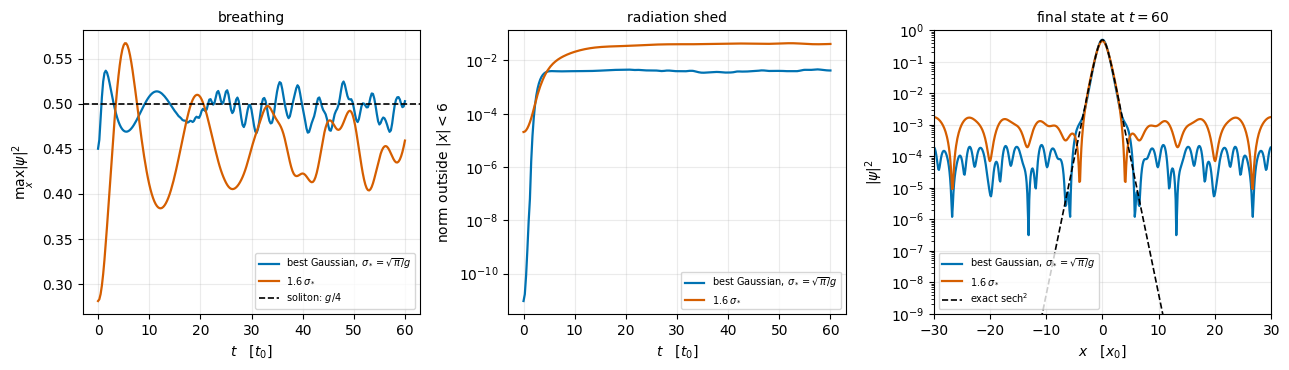
The right panel zooms on the two minima. The \(\mathrm{sech}\) family reaches \(-0.1667 = -g^{2}/24\) at \(\sigma = 0.9069\); the Gaussian family stops at \(-0.1592 = -g^{2}/(8\pi)\) at \(\sigma = 0.8862\). The best Gaussian overlaps the true soliton by \(0.9972\) — close, but Section 9.4 will show that the missing \(0.28\%\) is enough to make it breathe and radiate.

6.2 Collapse in one, two and three dimensions

Repeat the scaling argument in \(d\) dimensions. A normalised profile of width \(w\) has \(\vert\psi\vert^{2}\sim w^{-d}\), and the interaction integral \(\int\vert\psi\vert^{4}d^{d}x\) picks up \(w^{-2d}\cdot w^{d} = w^{-d}\), while the kinetic term is \(w^{-2}\) in any dimension:

\[ E_d(w) \;\sim\; \frac{a}{w^{2}} \;-\; \frac{b\,g}{w^{d}} . \]

• \(d=1\): the attraction, \(w^{-1}\), is weaker than the kinetic repulsion at small \(w\). A minimum exists at finite \(w\) for every \(g>0\). Solitons are stable, always.
• \(d=2\): both terms scale as \(w^{-2}\), so \(E_2(w) = (a-bg)/w^{2}\) and the sign of \(a-bg\) decides everything. For \(g\) below the critical value \(a/b\) the energy is positive and decreases towards zero as the cloud expands, so the minimiser runs off to \(w=\infty\); above it the energy is negative and runs to \(-\infty\) as \(w\to0\). There is no stable width at any \(g\) — the critical case, which is why two-dimensional attractive condensates are a delicate subject.
• \(d=3\): the attraction, \(w^{-3}\), beats the kinetic term at small \(w\), so \(E\to-\infty\) as \(w\to0\) for every \(g>0\): in free space a three-dimensional attractive condensate has no ground state at all. What produces a critical atom number is the trap that holds the cloud. Adding a harmonic trap of frequency \(\omega\) contributes \(+c\,\omega^{2}w^{2}\), and \(E(w) = a/w^{2} - bg/w^{3} + c\omega^{2}w^{2}\) has a local minimum at moderate \(w\) — a metastable condensate — separated by a barrier from the collapse at \(w\to0\). Increasing \(g\), i.e. increasing \(N\), lowers the barrier; at a critical \(N\) the local minimum and the barrier merge and disappear, and nothing stops the cloud from shrinking. The implosion, and the burst of atoms that escapes from it, was observed in \(^{85}\)Rb [14] and is called a Bosenova.

This is the reason every bright-soliton experiment starts by squeezing the gas into a waveguide: one dimension is the only dimension in which an attractive condensate has a ground state. Section 6.8 returns to the price of doing so in a real, three-dimensional trap.

6.3 A one-parameter family, and \(\mu = dE/dN\)

Equation (25) is a family labelled by the single combination \(ng\), i.e. by the number of atoms in the soliton:

quantity	scaling	in the physical units of Section 3
width	\(2/(ng)\)	\(\propto 1/N\)
peak amplitude	\(n\sqrt g/2\)	\(\propto N\)
peak density	\(n^{2}g/4\)	\(\propto N^{2}\)
chemical potential	\(-(ng)^{2}/8\)	\(\propto N^{2}\)
energy per particle	\(-(ng)^{2}/24\)	\(\propto N^{2}\)
total energy	\(n\cdot\left[-(ng)^{2}/24\right]\)	\(\propto N^{3}\)

More atoms means a narrower, taller, more deeply bound soliton, and the total energy falls as \(N^{3}\). The state is self-bound: \(\mu = -g^{2}/8 < 0\) means that removing one atom to rest at infinity costs energy \(g^{2}/8\), so the soliton holds itself together with no external trap. It is its own container.

The two energies of Section 4.5 are now related through the particle number. Restore the physical total energy of the cloud: by the unit table of Section 3.4, \(E_{\rm tot} = N E_0\,E[\psi]\), and \(g = cN\) with \(c = \vert g_{\rm 1D}\vert m x_0/\hbar^{2}\) fixed. Hence

\[ E_{\rm tot}(N) \;=\; N E_0\left(-\frac{c^{2}N^{2}}{24}\right) = -\frac{E_0c^{2}N^{3}}{24} \qquad\Longrightarrow\qquad \frac{dE_{\rm tot}}{dN} = -\frac{E_0c^{2}N^{2}}{8} = -E_0\frac{g^{2}}{8} = E_0\,\mu . \tag{32} \]

The chemical potential is the energy cost of adding one particle to the ground state — and it is the Lagrange multiplier that appeared in Eq. (5) precisely because it multiplies the constraint on \(N\). The cell below checks Eq. (32) in two independent ways: by automatic differentiation of the closed-form \(E_{\rm tot}(N)\), and by finite-differencing the numerically integrated energy of the exact profile.

JAX practice. jax.grad(f) returns a new function that computes the exact derivative of f by differentiating the operations f performs, not by taking finite differences — no step size, no truncation error. It is the tool that makes variational optimisation practical later in this course; see notebook 01, JAX.

Code

# ==============================================================================
# CHECKPOINT 3: mu = d E_tot / dN,  three ways
#   (a) jax.grad of the closed form  E_tot(N) = -c^2 N^3 / 24   (units of E_0)
#   (b) finite difference of  g -> g * E_numeric(g), with E_numeric integrated on the grid
#   (c) mu = <H_GP> on the exact profile        (already used in Checkpoint 1)
#   Choosing units with c = 1 makes g = N, so d/dN and d/dg are the same derivative.
# ==============================================================================
def total_energy_closed(N_atoms):
    """E_tot(N) / E_0 for a bright soliton, in units where g = N  (i.e. c = 1).

    MATH
        E_tot = N * E[psi] = N * (-g^2/24) = -N^3/24
    """
    return -N_atoms ** 3 / 24.0


mu_autodiff = float(jax.grad(total_energy_closed)(G))          # d E_tot / dN at N = g = G

h_g = 1e-4                                                     # finite-difference step in N = g
def total_energy_grid(g_val):
    """E_tot/E_0 = g * (energy per particle, integrated numerically over the exact profile)."""
    return g_val * gp_energy(soliton_exact(x, g=g_val), k, dx, g_val)

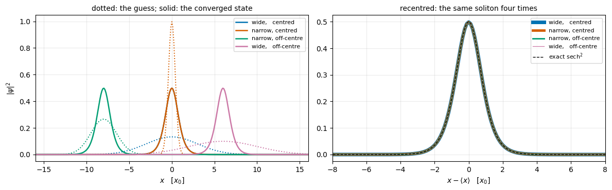
mu_fd = (total_energy_grid(G + h_g) - total_energy_grid(G - h_g)) / (2 * h_g)
mu_expect = gp_chemical_potential(soliton_exact(x, g=G), k, dx, G)

print(f"(a) jax.grad  of the closed form   : dE_tot/dN = {mu_autodiff:.12f}")
print(f"(b) finite difference of the grid E: dE_tot/dN = {mu_fd:.12f}   (h = {h_g:g})")
print(f"(c) mu = <H_GP> on the exact sech  : mu        = {mu_expect:.12f}")
print(f"    analytic -g^2/8                            = {-G ** 2 / 8:.12f}")
assert abs(mu_autodiff + G ** 2 / 8) < 1e4 * TOL
assert abs(mu_fd - mu_expect) < 1e-7, "finite-difference dE/dN must reproduce <H_GP>"
print("CHECKPOINT 3 passed: Eq. (32) holds.")

# a second, sharper statement of the same physics: the family scalings of the table above
print("\n  n g      width 2/(ng)   peak ampl.   mu = -(ng)^2/8    measured mu     measured width")
for n_frac in (0.5, 1.0, 2.0):
    psi_n = soliton_exact(x, g=G, n=n_frac)
    mu_meas = gp_chemical_potential(psi_n, k, dx, G) / grid_norm(psi_n, dx)
    w_predicted = 2.0 / (n_frac * G)
    # width read off the profile: sech(kappa d) = sech(1) at the distance d = 1/kappa = 2/(n g)
    i_peak = int(np.argmax(np.abs(psi_n)))
    prof = np.abs(psi_n)[i_peak:] / np.abs(psi_n)[i_peak]        # right half, monotonically decreasing
    j_cross = int(np.argmax(prof < 1.0 / np.cosh(1.0)))           # first sample below sech(1)
    w_meas = float(np.interp(1.0 / np.cosh(1.0), [prof[j_cross], prof[j_cross - 1]],
                             [x[i_peak + j_cross] - x[i_peak], x[i_peak + j_cross - 1] - x[i_peak]]))
    print(f"{n_frac * G:5.2f}   {w_predicted:12.6f} {n_frac * np.sqrt(G) / 2:12.6f} "
          f"{-(n_frac * G) ** 2 / 8:16.8f} {mu_meas:15.8f} {w_meas:18.6f}")

(a) jax.grad  of the closed form   : dE_tot/dN = -0.500000000000
(b) finite difference of the grid E: dE_tot/dN = -0.500000000418   (h = 0.0001)
(c) mu = <H_GP> on the exact sech  : mu        = -0.500000000000
    analytic -g^2/8                            = -0.500000000000
CHECKPOINT 3 passed: Eq. (32) holds.

  n g      width 2/(ng)   peak ampl.   mu = -(ng)^2/8    measured mu     measured width
 1.00       2.000000     0.353553      -0.12500000     -0.12500000           2.000050
 2.00       1.000000     0.707107      -0.50000000     -0.50000000           1.000350
 4.00       0.500000     1.414214      -2.00000000     -2.00000000           0.500704

All three routes to \(\mu\) agree: automatic differentiation of \(-N^{3}/24\), a finite difference of the grid energy, and the expectation value \(\langle \hat H_{\rm GP}\rangle\) all return \(-0.5 = -g^{2}/8\) for \(g=2\). The table underneath shows the family: doubling \(ng\) halves the width, doubles the amplitude and quadruples \(\vert\mu\vert\), and the measured width column — the distance from the peak at which the profile has fallen to \(\mathrm{sech}(1) = 0.6481\) of its maximum, obtained by linear interpolation between grid points — reproduces \(2/(ng)\) to a relative \(1.4\times10^{-3}\) or better, the interpolation error on a grid of spacing \(0.117\).

6.4 A soliton is a particle

Equation (26) says the soliton translates rigidly at velocity \(k_0\), and Eq. (28) says its energy is

\[ E \;=\; \underbrace{-\frac{g^{2}}{24}}_{\text{internal}} \;+\; \underbrace{\frac{k_0^{2}}{2}}_{\text{motion}} , \qquad \langle p\rangle = k_0 , \]

which is the energy of a particle of unit mass moving at velocity \(k_0\), plus a constant internal energy. In physical units the mass is \(Nm\): the whole cloud moves as one object. Combined with Ehrenfest’s relation (14) and \(d\langle p\rangle/dt = 0\), the centre of mass obeys Newton’s first law exactly, and because the shape never changes, so does every point of the profile.

The reason is Galilean invariance, and the reason that holds is that the nonlinearity depends only on \(\vert\psi\vert^{2}\), which no phase factor can touch. Adding an external potential breaks the invariance and the soliton then accelerates like a particle in that potential, which is what Ref. [4] observed when its solitons oscillated in a shallow axial trap (Exercise 1).

6.5 What the mean field hides: translational symmetry

Equation (8) is invariant under \(x\to x+x_c\), yet its solution (22) is localised at one particular \(x_c\) and therefore is not invariant. This is spontaneous symmetry breaking inside a variational ansatz, and it has a concrete consequence: the family of solitons at all \(x_c\) is degenerate, so the solution of an imaginary-time relaxation is determined entirely by where the initial guess happened to sit (Section 8.6 demonstrates this).

The many-body statement is sharper, and it is a genuine failure of the mean field rather than a technicality. The exact ground state of the \(N\)-boson Hamiltonian (2) with no external potential is an eigenstate of the total momentum and is therefore translationally invariant: the density of the exact ground state is uniform. What is localised is the relative wave function; the centre of mass of the soliton is completely delocalised, exactly as the centre of mass of a hydrogen atom in free space is. The Hartree product (3) cannot represent “localised internal structure with a delocalised centre of mass”, so it localises everything and produces a density profile that the exact ground state does not have. Ref. [19] constructed the corresponding exact quantum states, by the Bethe ansatz [20], for the quantum nonlinear Schrödinger model of solitons in optical fibres, which is the attractive one-dimensional Bose gas whose \(N\)-particle bound state had been found in [21]: superposing their momentum eigenstates with a wave packet in the total momentum recovers a localised density, which then spreads — a dispersive spreading of the centre of mass, as for a free particle of mass \(Nm\), that the Gross-Pitaevskii equation does not contain. Its size depends on the initial centre-of-mass uncertainty \(\Delta\), about which the mean field says nothing: the spread after a time \(t\) is \(\hbar t/(2Nm\Delta)\), which for \(N = 4.5\times10^{3}\) lithium atoms and \(t = 300\,\)ms is \(0.14\,\mu\)m if \(\Delta\) equals the soliton width \(\ell\) and \(10\,\mu\)m for the Hartree value \(\Delta = \sigma/\sqrt N\). A single absorption image does not show it either way: it records one localised soliton at a random position, and the spreading appears only as shot-to-shot scatter of that position.

6.6 Robustness, and integrability

A linear wave packet has no preferred shape: every initial condition spreads, and the spreading depends on which one you started from. The soliton is different. Start from a profile that is close to Eq. (22) and the state does not drift away: it oscillates about the soliton, sheds the mismatch as small-amplitude radiation that runs off, and settles onto a soliton. The soliton is an attractor of nearby initial conditions, in a system with no dissipation at all — the “dissipation” is radiation carrying the excess away from the core. Section 9.4 measures this for a Gaussian whose overlap with the soliton is \(0.9972\).

The deeper reason is that Eq. (8) is integrable. Ref. [22] showed that the nonlinear Schrödinger equation can be solved exactly by inverse scattering, the method introduced in [23] for the Korteweg-de Vries equation: one maps the initial condition to the scattering data of an auxiliary linear operator, evolves the scattering data trivially, and maps back. The equation possesses infinitely many independent conserved quantities — the norm, the momentum and the energy are only the first three — and its solutions decompose into solitons plus radiation, with the soliton content fixed for all time by the initial condition. That is why a perturbed soliton relaxes back to a soliton rather than to something else, and why two solitons pass through each other unchanged.

6.7 Where solitons matter

Optical fibres. Because Eq. (8) also governs a pulse envelope in a Kerr medium (Section 2.4), a light pulse of the right shape and peak power propagates down a fibre without broadening. Soliton transmission was proposed in [12] as the way to beat dispersion in long-haul communication, and soliton and dispersion-managed soliton systems were built and deployed; Ref. [24] (Chapter 5) gives the account.

Matter-wave interferometry. A soliton is a self-trapped, dispersionless, coherent matter wave, which makes it attractive as the moving arm of an atom interferometer: splitting, reflecting and recombining a soliton on a barrier keeps the packet compact for the whole interrogation time instead of letting it disperse. The stability of the soliton is doing work that a trap would otherwise have to do.

Soliton trains and modulational instability. A uniform attractive condensate is unstable against long-wavelength density modulations, the instability found in [25] for water waves: a small ripple grows because the region of higher density attracts more atoms. The instability breaks the cloud into a regular array of solitons. Ref. [4] proposed it as the origin of its train, and Ref. [26] characterised its role in train formation. The same instability, with the same equation, turns a continuous-wave laser beam in a fibre into a train of pulses [27].

6.8 Limits of validity of the one-dimensional description

Three assumptions were made, and each has a number attached.

1. Quasi-one-dimensionality. Reducing three dimensions to one requires every atom to stay in the transverse ground state, which needs the soliton to be longer than it is wide: \(\ell \gg a_\perp\), i.e. \(\kappa = N\vert a_s\vert/a_\perp = a_\perp/\ell \ll 1\). The cell in Section 3.5 gives \(\kappa = 0.66\) and \(0.60\) for the two experiments, which is of order one.
2. No collapse. The three-dimensional character reasserts itself when the soliton becomes narrow enough to feel the transverse degree of freedom, and then Section 6.2 applies: the cloud collapses. Numerical solutions of the full three-dimensional Gross-Pitaevskii equation in a waveguide put the threshold at \(\kappa_c = 0.675\pm0.005\) [28], in agreement with the analytic value \(2/3\) obtained in [29] from the non-polynomial Schrödinger equation of [30]. Both 2002 experiments therefore ran close to a genuine instability, which is why they could not simply increase \(N\) to make the soliton more one-dimensional: that is the direction in which it collapses. How close is a question the experiments themselves cannot answer sharply, because \(\kappa\) is linear in the atom number and \(N\) is the least precisely known quantity in the table. Ref. [3] measures \(N = 6(2)\times10^{3}\), whose central value gives \(\kappa = 0.88\) — above \(\kappa_c\) — while their own stability estimate, \(4.2\)–\(5.2\times10^{3}\), gives \(\kappa = 0.62\)–\(0.77\). The parameters used here, \(N = 4.5\times10^{3}\), sit inside that window. The experiment therefore operated at \(\kappa\) of order \(\kappa_c\), and the number that decides stability is the one with the largest error bar.
3. Mean field. Sections 2.3 and 6.5 listed what the Hartree product omits: quantum depletion, atoms outside the condensate mode, and the delocalisation of the centre of mass.

The cell below turns points 1 and 2 into numbers for the two experiments.

Code

# ==============================================================================
# CHECKPOINT 4: how close were the 2002 experiments to the collapse threshold?
#   kappa = N |a_s| / a_perp = a_perp / ell     (quasi-1D parameter)
#   kappa_c = 0.675 +/- 0.005                   (Ref. [28], 3D GP numerics)
# ==============================================================================
KAPPA_C = 0.675

print(f"{'experiment':24s} {'kappa':>8s} {'kappa/kappa_c':>14s} {'ell/a_perp':>12s} {'N_c':>8s}")
for name, N_at, a_s, nu in experiments:
    u = soliton_units(N_at, a_s, nu)
    n_crit = KAPPA_C * u["a_perp"] / abs(a_s)
    print(f"{name:24s} {u['kappa']:8.3f} {u['kappa'] / KAPPA_C:14.3f} {1 / u['kappa']:12.3f} {n_crit:8.0f}")
    assert u["kappa"] < KAPPA_C, "a published soliton must sit below the collapse threshold"
print("\nCHECKPOINT 4 passed: both experiments sit below kappa_c = 0.675, but not by much.")

# how sensitive is that verdict to the atom number?  kappa is LINEAR in N, and N carries the largest
# experimental error bar of the three inputs -- so the margin below kappa_c is only as good as N.
print("\nsensitivity to N (Ref. [3]: measured 6(2)e3, stability estimate 4.2-5.2e3):")
for N_try in (4200, 4500, 5200, 6000, 8000):
    print(f"    N = {N_try:5d}  ->  kappa = {soliton_units(N_try, -0.21e-9, 710.0)['kappa']:.3f}"
          f"   ({'below' if soliton_units(N_try, -0.21e-9, 710.0)['kappa'] < KAPPA_C else 'ABOVE'} kappa_c)")

experiment                  kappa  kappa/kappa_c   ell/a_perp      N_c
Ref. [3]                    0.663          0.983        1.507     4579
Ref. [4]                    0.596          0.883        1.677     5661

CHECKPOINT 4 passed: both experiments sit below kappa_c = 0.675, but not by much.

sensitivity to N (Ref. [3]: measured 6(2)e3, stability estimate 4.2-5.2e3):
    N =  4200  ->  kappa = 0.619   (below kappa_c)
    N =  4500  ->  kappa = 0.663   (below kappa_c)
    N =  5200  ->  kappa = 0.767   (ABOVE kappa_c)
    N =  6000  ->  kappa = 0.885   (ABOVE kappa_c)
    N =  8000  ->  kappa = 1.179   (ABOVE kappa_c)

7. Imaginary-time evolution

7.1 Ground states without diagonalisation

For a linear problem such as a harmonic trap, the ground state follows from building the Hamiltonian as a tridiagonal matrix and handing it to an eigensolver. That route is closed here for two independent reasons.

• \(\hat H_{\rm GP}[\psi]\) depends on \(\psi\). There is no fixed matrix to diagonalise; the “eigenvalue problem” (15) is nonlinear and an eigensolver has nothing to work on.
• Even for a linear problem, diagonalisation costs \(O(M^{3})\) time and \(O(M^{2})\) memory for a Hilbert space of dimension \(M\). For a grid of \(512\) points that is nothing; for the many-body Hilbert spaces of the later chapters, where \(M = 2^{20}\), it is impossible.

What follows is the standard replacement, and it needs nothing but the ability to apply \(\hat H\) to a state. As a grid method for the Schrödinger equation it is the relaxation method of [31]; for the Gross-Pitaevskii equation it was developed in [32].

7.2 The linear argument

Take a linear Hamiltonian \(\hat H\) with eigenstates \(\phi_n\) and energies \(E_0 \le E_1 \le E_2 \le\ldots\), and expand an arbitrary initial state,

\[ \psi(0) \;=\; \sum_n c_n\,\phi_n \qquad\Longrightarrow\qquad \psi(t) \;=\; \sum_n c_n\,e^{-iE_nt}\,\phi_n . \]

Every coefficient rotates; none decays; the state never settles. Now substitute

\[ t \;=\; -i\tau , \qquad \tau\in\mathbb{R},\ \tau>0 , \]

so that \(e^{-iE_nt} = e^{-iE_n(-i\tau)} = e^{-E_n\tau}\) and

\[ \psi(\tau) \;=\; \sum_n c_n\,e^{-E_n\tau}\,\phi_n \;=\; e^{-E_0\tau}\left[c_0\phi_0 \;+\; \sum_{n\ge1}c_n\,e^{-(E_n-E_0)\tau}\,\phi_n\right] . \tag{33} \]

The bracket is the whole argument. Every excited component is suppressed relative to the ground state by \(e^{-(E_n-E_0)\tau}\), and \(E_n - E_0 > 0\) for every \(n\) with \(E_n > E_0\). The prefactor \(e^{-E_0\tau}\) changes the norm — it shrinks it if \(E_0>0\), and grows it if \(E_0<0\), which is the case for our soliton — but it is a common factor and carries no information about the shape. Divide it out:

\[ \frac{\psi(\tau)}{\Vert\psi(\tau)\Vert} \;\xrightarrow[\tau\to\infty]{}\; \frac{\phi_0}{\Vert\phi_0\Vert} \qquad\text{provided } c_0 = \langle\phi_0\vert\psi(0)\rangle \ne 0 . \tag{34} \]

Three statements follow, and each is checked below.

1. Renormalise at every step. Not because the physics requires it, but because otherwise the numbers in the array run away exponentially. For the nonlinear problem there is a second reason: \(g\vert\psi\vert^{2}\) is only the physical interaction if \(\Vert\psi\Vert = 1\).
2. The convergence rate is the gap. The slowest-decaying contamination is the lowest excited state with \(c_n\ne0\), so the error falls as \(e^{-(E_1-E_0)\tau}\): a straight line on a semi-logarithmic plot, of measurable slope.
3. You get the lowest state with non-zero overlap, not necessarily the ground state. If a symmetry makes \(c_0\) vanish exactly, the method converges to the lowest state in the symmetry sector of the initial guess.

7.3 The algorithm: Strang splitting of \(e^{-\hat H\Delta\tau}\)

Applying \(e^{-\hat H\Delta\tau}\) requires a decision, because \(\hat H = \hat T + \hat W\) is a sum of two pieces that are easy separately and hard together:

\[ \hat T = -\frac{1}{2}\frac{\partial^{2}}{\partial x^{2}} \quad\text{(diagonal in Fourier space)}, \qquad \hat W = V(x) - g\vert\psi\vert^{2} \quad\text{(diagonal in position space)} . \]

They do not commute, so \(e^{-(\hat T+\hat W)h} \ne e^{-\hat Th}e^{-\hat Wh}\). Expanding both sides to second order,

\[ \begin{aligned} e^{-\hat Th}e^{-\hat Wh} &= 1 - h(\hat T+\hat W) + \frac{h^{2}}{2}\left(\hat T^{2} + 2\hat T\hat W + \hat W^{2}\right) + O(h^{3}) , \\ e^{-(\hat T+\hat W)h} &= 1 - h(\hat T+\hat W) + \frac{h^{2}}{2}\left(\hat T^{2} + \hat T\hat W + \hat W\hat T + \hat W^{2}\right) + O(h^{3}) , \end{aligned} \]

so the difference is \(\tfrac{h^{2}}{2}[\hat T,\hat W]\): the naive product is accurate only to first order in \(h\) per step. The cure is to symmetrise. Define the Strang product, introduced in [33],

\[ S(h) \;\equiv\; e^{-\hat Th/2}\;e^{-\hat Wh}\;e^{-\hat Th/2} . \tag{35} \]

Its error is one order better, and the proof needs no algebra at all. Reversing the sign of \(h\) reverses every factor and the order of the product is symmetric, so

\[ S(h)\,S(-h) = e^{-\hat Th/2}e^{-\hat Wh}e^{-\hat Th/2}\;e^{+\hat Th/2}e^{+\hat Wh}e^{+\hat Th/2} = 1 . \]

Writing \(S(h) = e^{-h\hat G(h)}\), this says \(\hat G(-h) = \hat G(h)\): the generator is an even function of \(h\), so it contains no \(h^{1}\) term,

\[ \hat G(h) \;=\; \hat T + \hat W + h^{2}\hat C_2 + O(h^{4}) . \tag{36} \]

The error per step is therefore \(O(h^{3})\), and over \(\tau/h\) steps the accumulated error is \(O(h^{2})\). The same \(S(h)\) with \(h\to i\,\Delta t\) is the real-time propagator of Section 9, where each of the three factors is separately unitary.

In practice the three factors are three lines of code — the split-step Fourier method, introduced for the Schrödinger equation in [34]:

\[ \psi \;\to\; \mathrm{IFFT}\left[e^{-k^{2}h/4}\,\mathrm{FFT}[\psi]\right] \;\to\; \psi\,e^{\left(g\vert\psi\vert^{2}-V\right)h} \;\to\; \mathrm{IFFT}\left[e^{-k^{2}h/4}\,\mathrm{FFT}[\psi]\right] \;\to\; \frac{\psi}{\Vert\psi\Vert} . \tag{37} \]

The exponent of the kinetic half-step is \(-\tfrac{k^{2}}{2}\cdot\tfrac{h}{2} = -k^{2}h/4\); the sign in the middle factor is positive for \(g>0\) because attraction lowers the energy and imaginary time amplifies whatever lowers the energy.

Code

# ==============================================================================
# STEP 3: imaginary-time propagation by Strang split-step  -- Eq. (37)
#   One scan body, two entry points:
#     imaginary_time_ground_state : run n_steps and return the final state + the norm of each step
#     imaginary_time_frames       : the same, but keep a snapshot every n_inner steps (for movies)
# ==============================================================================
def _imag_step_factory(k, dx, g, V, dtau):
    """Build the one-step map of Eq. (37) for fixed parameters (used by both entry points)."""
    exp_kin = jnp.exp(-0.25 * k ** 2 * dtau)             # exp(-(k^2/2)(dtau/2)), the kinetic HALF step

    def step(psi, _):
        psi = jnp.fft.ifft(exp_kin * jnp.fft.fft(psi))               # kinetic half step
        psi = psi * jnp.exp((g * jnp.abs(psi) ** 2 - V) * dtau)      # nonlinear + potential full step
        psi = jnp.fft.ifft(exp_kin * jnp.fft.fft(psi))               # kinetic half step
        nrm = jnp.sqrt(dx * jnp.sum(jnp.abs(psi) ** 2))              # imaginary time does NOT conserve the norm
        return psi / nrm, nrm                                        # (carry, per-step norm)
    return step


@partial(jax.jit, static_argnames=("n_steps",))
def imaginary_time_ground_state(psi, k, dx, g, V, dtau, n_steps):
    """Relax psi towards the lowest state of H_GP by n_steps of Eq. (37).

    MATH
        psi <- N[ exp(-T dtau/2) exp(-W dtau) exp(-T dtau/2) psi ],  W = V - g|psi|^2
    RETURNS
        (psi, norms) with norms[j] = || psi ||  BEFORE the renormalisation of step j.
        Section 7.9 reads the chemical potential off those norms.
    COST
        2 FFTs of length N_x per step, i.e. O(N_x log N_x); memory O(N_x).
    JAX
        lax.scan compiles the loop body ONCE instead of unrolling n_steps copies of it.
    """
    return lax.scan(_imag_step_factory(k, dx, g, V, dtau), psi, None, length=n_steps)


@partial(jax.jit, static_argnames=("n_inner", "n_frames"))
def imaginary_time_frames(psi, k, dx, g, V, dtau, n_inner, n_frames):
    """Same relaxation, keeping a snapshot every n_inner steps. Shape (n_frames+1, N_x), frame 0 = input."""
    step = _imag_step_factory(k, dx, g, V, dtau)

    def outer(psi, _):
        psi, _ = lax.scan(step, psi, None, length=n_inner)
        return psi, psi

    _, frames = lax.scan(outer, psi, None, length=n_frames)
    return jnp.concatenate([psi[None, :], frames], axis=0)


print("STEP 3: imaginary_time_ground_state and imaginary_time_frames compiled on first call.")

STEP 3: imaginary_time_ground_state and imaginary_time_frames compiled on first call.

JAX practice. jax.jit compiles a Python function once, for the shapes of its arguments, into a single fused program; lax.scan(body, init, xs, length=n) is a compiled for loop that carries a state forward and collects one output per iteration. Marking n_steps as a static argument tells the compiler that this number is known at compile time, which it must be for scan to fix the loop length; changing it triggers a recompilation. Both are explained in notebook 01, JAX.

7.4 Demonstration 1: the convergence rate is the gap

The place to test the machinery is a problem where every answer is known: the harmonic oscillator \(V(x) = x^{2}/2\), with \(E_n = n+\tfrac12\), ground state \(\phi_0 = \pi^{-1/4}e^{-x^{2}/2}\), and a gap \(E_1-E_0 = 1\). Setting \(g = 0\) in Eq. (37) makes it a purely linear calculation.

The initial guess is a Gaussian of the wrong width placed off centre, so that it has non-zero overlap with every eigenstate. Equation (33) then predicts

\[ \left\Vert \frac{\psi(\tau)}{\Vert\psi(\tau)\Vert} - \phi_0 \right\Vert \;\propto\; e^{-(E_1-E_0)\tau} \;=\; e^{-\tau} , \]

a straight line of slope \(-1\) on a semi-logarithmic plot. If instead the guess is placed at the centre, parity makes \(c_1 = c_3 = \ldots = 0\) exactly, the slowest surviving contamination is \(\phi_2\), and the slope must be \(-(E_2-E_0) = -2\).

Code

# ==============================================================================
# PARAMETERS for the linear harmonic-oscillator demonstrations of Section 7
# ==============================================================================
L_HO, N_HO = 24.0, 256
x_ho, k_ho, dx_ho = make_grid(L_HO, N_HO)
V_HO = jnp.asarray(0.5 * x_ho ** 2)                    # the harmonic trap V = x^2/2, in oscillator units
k_ho_j = jnp.asarray(k_ho)
V_HO_np = np.asarray(V_HO)

DTAU_HO = 0.005                                        # small enough that the splitting bias is invisible here
phi0_ho = (np.pi ** -0.25) * np.exp(-x_ho ** 2 / 2)    # exact ground state
phi1_ho = np.sqrt(2.0) * (np.pi ** -0.25) * x_ho * np.exp(-x_ho ** 2 / 2)
phi2_ho = (np.pi ** -0.25) / np.sqrt(2.0) * (2 * x_ho ** 2 - 1) * np.exp(-x_ho ** 2 / 2)

print(f"harmonic-oscillator grid: L = {L_HO}, N_x = {N_HO}, dx = {dx_ho:.5f}, dtau = {DTAU_HO}")
print(f"exact levels E_n = n + 1/2; gap E_1 - E_0 = 1, E_2 - E_0 = 2")

harmonic-oscillator grid: L = 24.0, N_x = 256, dx = 0.09375, dtau = 0.005
exact levels E_n = n + 1/2; gap E_1 - E_0 = 1, E_2 - E_0 = 2

Code

# ==============================================================================
# DEMONSTRATION 1: the error decays at the rate of the gap
# ==============================================================================
TAU_STEP, N_TAU = 0.25, 60                             # snapshots every 0.25 up to tau = 15
n_inner_ho = int(round(TAU_STEP / DTAU_HO))
taus_ho = np.arange(N_TAU + 1) * TAU_STEP

guesses = {"off-centre Gaussian (all $n$)": gaussian_packet(x_ho, 0.7, x_c=1.5),
           "centred Gaussian (even $n$ only)": gaussian_packet(x_ho, 0.7, x_c=0.0)}

fig, axes = plt.subplots(1, 2, figsize=(12.0, 4.0))
fit_slopes, errs_final, ens_final = {}, {}, {}
for label, psi_start in guesses.items():
    psi_start = jnp.asarray(normalise(psi_start, dx_ho))
    frames = np.asarray(imaginary_time_frames(psi_start, k_ho_j, dx_ho, 0.0, V_HO,
                                              DTAU_HO, n_inner_ho, N_TAU))
    # global phase is irrelevant: compare the amplitudes
    errs = np.array([np.sqrt(dx_ho * np.sum((np.abs(f) - phi0_ho) ** 2)) for f in frames])
    ens = np.array([gp_energy(f, k_ho, dx_ho, 0.0, V_HO_np) for f in frames])
    # fit only where the error is still falling: below ~100 times its own floor the curve is
    # dominated by the O(dtau^2) bias of the splitting, not by the spectral gap (Section 8.2)
    window = (taus_ho >= 1.0) & (errs > 100.0 * errs.min())
    slope = np.polyfit(taus_ho[window], np.log(errs[window]), 1)[0]
    fit_slopes[label], errs_final[label], ens_final[label] = slope, errs[-1], ens[-1] - 0.5
    axes[0].semilogy(taus_ho, errs, lw=1.8, label=f"{label}: slope {slope:.3f}")
    axes[1].plot(taus_ho, ens - 0.5, lw=1.8, label=label)

axes[0].semilogy(taus_ho, 0.35 * np.exp(-taus_ho), "k--", lw=1.0, label=r"$e^{-\tau}$ (gap $=1$)")
axes[0].semilogy(taus_ho, 0.20 * np.exp(-2 * taus_ho), "k:", lw=1.0, label=r"$e^{-2\tau}$ (gap $=2$)")
axes[0].set_xlabel(r"$\tau$   [$1/\omega_0$]"), axes[0].set_ylabel(r"$\Vert\,|\psi(\tau)|-\phi_0\Vert$")
axes[0].set_ylim(1e-8, 3), axes[0].grid(alpha=0.25), axes[0].legend(fontsize=8)
axes[0].set_title("distance to the exact ground state", fontsize=10)
axes[1].set_yscale("log")
axes[1].set_xlabel(r"$\tau$   [$1/\omega_0$]"), axes[1].set_ylabel(r"$E(\tau)-E_0$   [$\hbar\omega_0$]")
axes[1].grid(alpha=0.25), axes[1].legend(fontsize=8)
axes[1].set_title(r"the energy falls to $E_0=1/2$ and stops at the $\Delta\tau^2$ bias", fontsize=10)
fig.tight_layout()
plt.show()

for label, slope in fit_slopes.items():
    print(f"{label:36s} fitted decay rate = {slope:7.4f}")
print(f"plateau of the state error at tau = {taus_ho[-1]:g}: {errs_final['off-centre Gaussian (all $n$)']:.2e} "
      f"and {errs_final['centred Gaussian (even $n$ only)']:.2e}")
print(f"plateau of the energy error                : {ens_final['off-centre Gaussian (all $n$)']:.2e} "
      f"and {ens_final['centred Gaussian (even $n$ only)']:.2e}   (the O(dtau^2) bias at dtau = {DTAU_HO})")
assert abs(fit_slopes["off-centre Gaussian (all $n$)"] + 1.0) < 0.02, "rate must equal the gap E_1 - E_0 = 1"
assert abs(fit_slopes["centred Gaussian (even $n$ only)"] + 2.0) < 0.05, "parity doubles the rate"
print("\nCHECKPOINT 5 passed: the imaginary-time convergence rate is the spectral gap.")

off-centre Gaussian (all $n$)        fitted decay rate = -0.9990
centred Gaussian (even $n$ only)     fitted decay rate = -2.0193
plateau of the state error at tau = 15: 1.15e-06 and 1.10e-06
plateau of the energy error                : 2.55e-12 and 2.44e-12   (the O(dtau^2) bias at dtau = 0.005)

CHECKPOINT 5 passed: the imaginary-time convergence rate is the spectral gap.

The off-centre guess decays with fitted rate \(-0.999\); the predicted rate is \(-(E_1-E_0) = -1\). The centred guess decays at \(-2.02\) against the predicted \(-(E_2-E_0) = -2\) — parity removes every odd eigenstate from the expansion, so the first surviving contamination is \(\phi_2\) and the convergence is twice as fast.

Both curves stop on a plateau at \(1.1\times10^{-6}\) rather than continuing to zero. That plateau is not a failure of the argument: it is the \(O(\Delta\tau^{2})\) bias of the split-step map at \(\Delta\tau = 0.005\), and Section 8.2 measures it. The fit window above therefore excludes everything within a factor \(100\) of it; fitting through the plateau would return a meaningless slope.

The right panel shows the energy falling towards \(E_0 = 1/2\), as Section 7.7 will show it must. Its plateau is at \(2.5\times10^{-12}\), six orders below the plateau of the state, which is the variational effect that Section 8.2 explains: an error \(\varepsilon\) in the state costs only \(O(\varepsilon^{2})\) in the energy.

The centred guess starts much closer to \(\phi_0\) than the off-centre one, and its energy curve does something the monotonicity argument of Section 7.7 appears to forbid: it dips to \(1\times10^{-13}\) at \(\tau\approx4.5\) and climbs back to the plateau at \(2.4\times10^{-12}\). Nothing is wrong. Equation (40) is a statement about the continuous flow (39); what the code iterates is the discrete map (37), which decreases the energy of the modified generator (36), not of \(\hat H\) itself. The two differ by \(O(\Delta\tau^{2})\) — exactly the size of the plateau — so the measured \(E(\tau)\) is guaranteed to fall only until it reaches that level. Above the bias the descent is monotonic; at the bias the curve is free to wander inside it.

7.5 Demonstration 2: convergence to the lowest state with non-zero overlap

Start instead from an odd function, \(\psi(x,0)\propto x\,e^{-x^{2}/4s^{2}}\). Parity is a symmetry of the Hamiltonian, and every operation in Eq. (37) preserves it — the FFT of an odd array is odd, multiplication by the even \(V\) keeps it odd — so \(c_0 = c_2 = \ldots = 0\) for ever, in exact arithmetic. Equation (33) then converges to \(\phi_1\), the first excited state, and the method returns \(E = 3/2\).

In floating-point arithmetic “for ever” means “until round-off”. Every step introduces an even component of relative size \(\varepsilon\sim10^{-16}\), and each such component then grows relative to the odd one by \(e^{(E_1-E_0)\tau} = e^{\tau}\). Summed over the \(\tau/\Delta\tau\) steps, the contamination at time \(\tau\) is about \(\varepsilon e^{\tau}/\Delta\tau\), which reaches order one at \(\tau\approx\ln(\Delta\tau/\varepsilon)\approx31\) for \(\Delta\tau = 0.005\). The calculation below runs well past that point.

Code

# ==============================================================================
# DEMONSTRATION 2: an odd initial guess converges to phi_1 -- until round-off wins
# ==============================================================================
psi_odd = jnp.asarray(normalise((x_ho * np.exp(-x_ho ** 2 / (4 * 0.7 ** 2))).astype(CDTYPE), dx_ho))

print(f"{'tau':>6s} {'E(tau)':>14s} {'|<phi_0|psi>|':>15s} {'|<phi_1|psi>|':>15s}   state")
tau_list = [5.0, 10.0, 20.0, 30.0, 35.0, 40.0, 50.0, 70.0]
overlaps0 = []
for tau_end in tau_list:
    psi_t, _ = imaginary_time_ground_state(psi_odd, k_ho_j, dx_ho, 0.0, V_HO,
                                           DTAU_HO, int(round(tau_end / DTAU_HO)))
    p = np.asarray(psi_t)
    o0 = abs(dx_ho * np.sum(phi0_ho * np.conj(p)))
    o1 = abs(dx_ho * np.sum(phi1_ho * np.conj(p)))
    e_t = gp_energy(p, k_ho, dx_ho, 0.0, V_HO_np)
    overlaps0.append(o0)
    print(f"{tau_end:6.1f} {e_t:14.9f} {o0:15.3e} {o1:15.3e}   "
          f"{'first excited' if o1 > o0 else 'ground state'}")

assert overlaps0[0] < 1e-8 and overlaps0[-1] > 0.999, \
    "the odd guess must sit on phi_1 first and collapse to phi_0 later"
print("\nCHECKPOINT 6 passed: symmetry protects the excited state, round-off eventually destroys it.")

   tau         E(tau)   |<phi_0|psi>|   |<phi_1|psi>|   state
   5.0    1.500000000       1.237e-12       1.000e+00   first excited
  10.0    1.500000000       1.849e-10       1.000e+00   first excited

  20.0    1.500000000       4.073e-06       1.000e+00   first excited
  30.0    1.492014620       8.936e-02       9.960e-01   first excited

  35.0    0.505608408       9.972e-01       7.489e-02   ground state
  40.0    0.500000256       1.000e+00       5.060e-04   ground state

  50.0    0.500000000       1.000e+00       2.297e-08   ground state

  70.0    0.500000000       1.000e+00       8.440e-15   ground state

CHECKPOINT 6 passed: symmetry protects the excited state, round-off eventually destroys it.

From \(\tau = 5\) to \(\tau = 20\) the state is \(\phi_1\) and the energy is \(3/2\) to nine digits: the algorithm has converged to an excited state, because the ground state was not in the initial expansion. The even contamination is \(1.2\times10^{-12}\) at \(\tau=5\), \(1.8\times10^{-10}\) at \(\tau=10\) and \(4.1\times10^{-6}\) at \(\tau=20\), growth by \(e^{\tau}\) to within \(1\%\) over fifteen units of \(\tau\); the value at \(\tau = 5\) is within a factor of three of the estimate \(\varepsilon e^{5}/\Delta\tau = 3\times10^{-12}\). By \(\tau = 30\) it is \(8.9\%\), at \(\tau = 35\) the state has flipped, and from \(\tau = 40\) on the energy is \(1/2\) and the overlap with \(\phi_0\) is one.

Common pitfall. “Imaginary time converges to the ground state” is false as stated. It converges to the lowest state that the initial guess overlaps, and in a symmetric problem a symmetric guess can miss the ground state entirely — silently, with a perfectly converged-looking energy. Always check the state, not just the energy, and when in doubt break the symmetry of the guess on purpose (or add noise, as Section 8.6 does).

7.6 Excited states by projection

The same observation turns into a method. If \(\phi_0\) is already known, run the relaxation while projecting it out after every step,

\[ \psi \;\to\; \psi \;-\; \phi_0\,\langle\phi_0\vert\psi\rangle , \]

which is one Gram-Schmidt sweep. The component along \(\phi_0\) is removed faster than it can regrow, the expansion (33) starts at \(n=1\), and the relaxation converges to \(\phi_1\) at rate \(E_2-E_1\). Projecting out \(\phi_0\) and \(\phi_1\) gives \(\phi_2\), and so on. The cost of each additional state is one more inner product per step.

Code

# ==============================================================================
# DEMONSTRATION 3: the first three oscillator states by imaginary time + Gram-Schmidt
# ==============================================================================
@partial(jax.jit, static_argnames=("n_steps",))
def imaginary_time_excited(psi, k, dx, V, dtau, n_steps, basis):
    """Imaginary-time relaxation with the rows of `basis` projected out after every step (linear H only).

    MATH
        psi <- N[ P (exp(-T dt/2) exp(-V dt) exp(-T dt/2) psi) ],   P = 1 - sum_m |b_m><b_m|
    IMPLEMENTATION
        <b_m|psi> = dx sum_j conj(b_m)_j psi_j  -> one matrix-vector product per step.
    """
    exp_kin = jnp.exp(-0.25 * k ** 2 * dtau)

    def step(psi, _):
        psi = jnp.fft.ifft(exp_kin * jnp.fft.fft(psi))
        psi = psi * jnp.exp(-V * dtau)
        psi = jnp.fft.ifft(exp_kin * jnp.fft.fft(psi))
        psi = psi - basis.T @ (dx * (jnp.conj(basis) @ psi))          # remove the known states
        return psi / jnp.sqrt(dx * jnp.sum(jnp.abs(psi) ** 2)), None

    return lax.scan(step, psi, None, length=n_steps)[0]


rng = np.random.default_rng(20260919)
start_noisy = normalise((np.exp(-x_ho ** 2 / 4) * (1.0 + 0.3 * rng.standard_normal(N_HO))).astype(CDTYPE), dx_ho)

found, exact_states = [], [phi0_ho, phi1_ho, phi2_ho]
print(f"{'n':>2s} {'E_n numerical':>16s} {'E_n exact':>11s} {'error':>10s} {'|<phi_n|psi_n>|':>17s}")
for n_state in range(3):
    basis_j = (jnp.asarray(np.array(found)) if found
               else jnp.zeros((0, N_HO), dtype=CDTYPE))
    psi_n = np.asarray(imaginary_time_excited(jnp.asarray(start_noisy), k_ho_j, dx_ho, V_HO,
                                              DTAU_HO, int(round(30.0 / DTAU_HO)), basis_j))
    found.append(psi_n)
    e_n = gp_energy(psi_n, k_ho, dx_ho, 0.0, V_HO_np)
    ov = abs(dx_ho * np.sum(np.conj(exact_states[n_state]) * psi_n))
    print(f"{n_state:2d} {e_n:16.10f} {n_state + 0.5:11.1f} {abs(e_n - n_state - 0.5):10.2e} {ov:17.10f}")
    assert abs(e_n - (n_state + 0.5)) < 1e-6 and ov > 1 - 1e-6

print("\nCHECKPOINT 7 passed: imaginary time + Gram-Schmidt reproduces E_n = n + 1/2.")

 n    E_n numerical   E_n exact      error   |<phi_n|psi_n>|
 0     0.5000000000         0.5   2.44e-12      1.0000000000

 1     1.5000000000         1.5   7.32e-12      1.0000000000
 2     2.5000000000         2.5   1.22e-11      1.0000000000

CHECKPOINT 7 passed: imaginary time + Gram-Schmidt reproduces E_n = n + 1/2.

Three runs of the same loop, each \(\tau=30\) long, return \(0.5\), \(1.5\) and \(2.5\) to ten digits and the corresponding Hermite functions to an overlap of \(1\). The initial guess was a noisy Gaussian with no symmetry at all, so nothing here relies on parity: the projection does the work.

This is how excited states are obtained without diagonalisation. Its cost per state is one extra inner product per step; its weakness is that errors in \(\phi_0\) propagate into \(\phi_1\), so the accuracy degrades as one climbs.

7.7 Three ways to look at the same algorithm

Equation (33) is one derivation. Three more points of view explain different aspects of the method, and the third is the only one that survives the nonlinearity.

(a) A diffusion equation with absorption. Written out, \(\partial_\tau\psi = -\hat H\psi\) reads

\[ \frac{\partial\psi}{\partial\tau} \;=\; \frac{1}{2}\frac{\partial^{2}\psi}{\partial x^{2}} \;-\; V(x)\,\psi , \tag{38} \]

which is a diffusion equation with a position-dependent sink. The Laplacian smooths \(\psi\) — it destroys sharp features, short wavelengths decaying fastest, at rate \(k^{2}/2\) — while the term \(-V\psi\) removes amplitude fastest where the potential is large. The competition between smoothing and selective absorption sculpts the ground state: smooth, and concentrated where \(V\) is small. The kinetic half-steps of Eq. (37) are exactly a diffusion step in Fourier space, and the middle factor is exactly the absorption. For an attractive nonlinearity the sink becomes a source, \(-W = g\vert\psi\vert^{2} > 0\): amplitude grows where there is already amplitude, which is self-focusing in one line.

(b) The power method. One step of Eq. (37) is multiplication by the fixed operator \(M = e^{-\hat H\Delta\tau}\) followed by renormalisation. That is the power method of [35] for finding the dominant eigenvector of a matrix. The eigenvalues of \(M\) are \(e^{-E_n\Delta\tau}\), and the largest of them belongs to the lowest energy — the exponential turns “smallest eigenvalue of \(\hat H\)” into “largest eigenvalue of \(M\)”, which is what a power method can find. The convergence ratio per step is \(e^{-(E_1-E_0)\Delta\tau}\), which is Eq. (33) again, and the dominant eigenvalue itself is read off the norm ratio (Section 7.9). The only reason we never form \(M\) as a matrix is that applying it costs two FFTs while storing it would cost \(N_x^{2}\) numbers.

(c) Steepest descent on the energy functional. Renormalising after every step keeps the state on the unit sphere \(\Vert\psi\Vert = 1\). The combination of an unconstrained step \(-\hat H_{\rm GP}\psi\,\Delta\tau\) and the projection back onto the sphere is, to first order in \(\Delta\tau\), a step along

\[ \frac{\partial\psi}{\partial\tau} \;=\; -\left(\hat H_{\rm GP}[\psi] - \mu[\psi]\right)\psi , \qquad \mu[\psi] = \int\psi^{*}\hat H_{\rm GP}[\psi]\,\psi\;dx , \tag{39} \]

where \(\mu\) is precisely the Lagrange multiplier that enforces \(\Vert\psi\Vert=1\): the term \(+\mu\psi\) removes the component of the gradient along \(\psi\), which is the one that would change the norm. This is gradient descent on \(E[\psi]\) restricted to the sphere. Repeating the three lines of Section 4.3 with \(-i\hat H\) replaced by \(-(\hat H_{\rm GP}-\mu)\):

\[ \begin{aligned} \frac{dE}{d\tau} &= 2\,\mathrm{Re}\int\left(\hat H_{\rm GP}\psi\right)\frac{\partial\psi^{*}}{\partial\tau}\,dx = -2\,\mathrm{Re}\int\left(\hat H_{\rm GP}\psi\right) \left(\hat H_{\rm GP}\psi - \mu\psi\right)^{*}dx \\ &= -2\left[\int\left\vert \hat H_{\rm GP}\psi\right\vert^{2}dx - \mu^{2}\right] = -2\left\Vert\left(\hat H_{\rm GP}-\mu\right)\psi\right\Vert^{2} \;\le\; 0 , \end{aligned} \tag{40} \]

using \(\mu\) real and \(\int(\hat H_{\rm GP}\psi)\psi^{*} = \mu\) in the third step, and \(\Vert(\hat H-\mu)\psi\Vert^{2} = \Vert \hat H\psi\Vert^{2} - 2\mu\cdot\mu + \mu^{2} = \Vert \hat H\psi\Vert^{2}-\mu^{2}\) in the fourth.

Equation (40) is the algorithm’s guarantee. The energy never increases; it stops decreasing exactly when the residual \(\Vert(\hat H_{\rm GP}-\mu)\psi\Vert\) vanishes, and that is the stationary equation (15). The residual is therefore both the convergence monitor and the speed of descent, and the two are tied together by a formula we can test.

The guarantee belongs to the continuous flow (39). A discrete step of size \(\Delta\tau\) inherits it only down to the \(O(\Delta\tau^{2})\) level at which the map (37) stops being that flow — which is why the energy curves below are monotonic while they are falling and flat, not monotonic, once they reach their bias.

Code

# ==============================================================================
# DEMONSTRATION 4: the energy really is a gradient flow -- Eq. (40) measured
#   dE/dtau is estimated by a centred difference along a stored trajectory,
#   and compared with -2 * residual^2 computed independently at the same tau.
# ==============================================================================
TAU_SNAP, N_SNAP = 0.02, 100
DTAU_FLOW = 0.001

fig, axes = plt.subplots(1, 2, figsize=(12.0, 4.0))
for ax, (tag, Lg, Ng, gg, Vg, start) in zip(axes, [
        ("linear: harmonic trap", L_HO, N_HO, 0.0, lambda xx: 0.5 * xx ** 2,
         lambda xx: gaussian_packet(xx, 0.7, x_c=1.5)),
        ("nonlinear: bright soliton", L, N_X, G, lambda xx: 0.0 * xx,
         lambda xx: gaussian_packet(xx, 3.0))]):
    xg, kg, dxg = make_grid(Lg, Ng)
    Vg_np = Vg(xg)
    psi_s = jnp.asarray(normalise(start(xg), dxg))
    fr = np.asarray(imaginary_time_frames(psi_s, jnp.asarray(kg), dxg, gg, jnp.asarray(Vg_np),
                                          DTAU_FLOW, int(round(TAU_SNAP / DTAU_FLOW)), N_SNAP))
    tau_s = np.arange(N_SNAP + 1) * TAU_SNAP
    E_s = np.array([gp_energy(f, kg, dxg, gg, Vg_np) for f in fr])
    R_s = np.array([gp_residual(f, kg, dxg, gg, Vg_np) for f in fr])
    dE_measured = (E_s[2:] - E_s[:-2]) / (2 * TAU_SNAP)
    dE_predicted = -2.0 * R_s[1:-1] ** 2
    rel = np.max(np.abs(dE_measured - dE_predicted) / np.abs(dE_predicted))
    ax.plot(tau_s[1:-1], -dE_measured, color=C_NUM, lw=2.2, label=r"$-dE/d\tau$ (finite difference)")
    ax.plot(tau_s[1:-1:3], 2 * R_s[1:-1:3] ** 2, "o", ms=4, color=C_ANA, mfc="none",
            label=r"$2\Vert(\hat H_{\rm GP}-\mu)\psi\Vert^{2}$")
    ax.set_yscale("log"), ax.grid(alpha=0.25)
    ax.set_xlabel(r"$\tau$"), ax.set_ylabel(r"$-dE/d\tau$")
    ax.set_title(f"{tag}: max relative deviation {rel:.1e}", fontsize=10)
    ax.legend(fontsize=8)
    assert np.all(np.diff(E_s) <= 1e-14), "the energy must never increase"
    assert rel < 5e-3, "Eq. (40) must hold to the accuracy of the finite difference in tau"
    print(f"{tag:28s}: E decreases monotonically from {E_s[0]:+.6f} to {E_s[-1]:+.6f}; "
          f"Eq. (40) holds to {rel:.1e}")
fig.tight_layout()
plt.show()
print("\nCHECKPOINT 8 passed: imaginary time is normalised gradient flow, Eq. (40).")

linear: harmonic trap       : E decreases monotonically from +1.625102 to +0.521016; Eq. (40) holds to 2.7e-04
nonlinear: bright soliton   : E decreases monotonically from -0.080143 to -0.095788; Eq. (40) holds to 2.8e-04

CHECKPOINT 8 passed: imaginary time is normalised gradient flow, Eq. (40).

Both panels put two independently computed quantities on top of each other: the numerical derivative of the stored energy curve, and twice the squared residual evaluated from the stored states. They agree to \(2.7\times10^{-4}\) (linear) and \(2.8\times10^{-4}\) (nonlinear), which is the truncation error of the centred difference with \(\Delta\tau_{\rm snap}=0.02\), not a discrepancy in Eq. (40). The energy is monotonic in both runs. Over the two units of \(\tau\) plotted, the linear descent rate falls by a factor \(50\) while the nonlinear one rises by \(45\%\): gradient flow is not obliged to slow down monotonically, only to keep \(dE/d\tau\le0\), and the wide Gaussian of the right panel is still accelerating into the minimum at \(\tau = 2\).

7.8 What changes when the equation is nonlinear

The derivation of Section 7.2 uses the superposition principle twice: to expand \(\psi\) in eigenstates and to evolve each term independently. Neither step is available for Eq. (8). There is no eigenbasis of \(\hat H_{\rm GP}[\psi]\) that does not itself depend on \(\psi\), and \(e^{-\hat H_{\rm GP}\tau}\) applied to a sum is not the sum of the results.

What survives is viewpoint (c). Equations (39) and (40) never used linearity: they used only that \(E[\psi]\) is a real functional and that \(\hat H_{\rm GP}\psi = \delta E/\delta\psi^{*}\). So for the Gross-Pitaevskii equation, imaginary-time relaxation is normalised gradient flow of the energy functional, and it is guaranteed to decrease \(E\) until the residual vanishes. Ref. [36] proved that this continuous normalised gradient flow conserves the norm and diminishes the energy, and analysed discretisations of it in which the normalisation is applied after each step.

Three consequences of replacing “lowest eigenstate” by “local minimum of a functional”:

• “Ground state” now means “minimiser of \(E[\psi]\) at fixed norm”. For the attractive one-dimensional problem that minimiser exists and is unique up to translation and a global phase (Section 6.2), so the distinction is academic here. For a condensate in a double well, a rotating trap or a spinor gas it is not: the energy landscape has several local minima, and gradient flow finds the one whose basin contains the initial guess.
• The initial guess matters more than in the linear case. It decides the basin, and — through the zero mode of translation — it decides where the soliton ends up (Section 8.6).
• \(\mu\) is a Lagrange multiplier, not an eigenvalue. It appears in Eq. (39) to enforce the constraint, and it equals \(\langle \hat H_{\rm GP}\rangle\) only at the fixed point. Away from it, \(\mu[\psi]\) and \(E[\psi]\) are two different numbers, both changing.

7.9 Reading \(\mu\) off the norm decay

Near the fixed point the step of Eq. (37) acts on \(\psi_{*}\) like \(e^{-\hat H_{\rm GP}\Delta\tau}\) acting on its own eigenstate, so the unnormalised output is

\[ S(\Delta\tau)\,\psi_{*} \;=\; e^{-\mu\Delta\tau}\,\psi_{*} + O(\Delta\tau^{3}) . \]

At the fixed point of the discrete map the output is exactly proportional to \(\psi_{*}\), so the relation below defines a number for any \(\Delta\tau\); how close that number is to \(\mu\) is a separate question, and the \(O(\Delta\tau^{3})\) above is the linear-problem answer. Since the state entering each step has unit norm, the norm recorded before the renormalisation is \(\nu = e^{-\mu\Delta\tau}\), and therefore

\[ \mu \;=\; -\,\frac{\ln \nu}{\Delta\tau} \;=\; -\,\frac{\ln\left(\nu^{2}\right)}{2\,\Delta\tau} . \tag{41} \]

This costs nothing — the norm has to be computed anyway to renormalise — and it is completely independent of the expectation value \(\langle \hat H_{\rm GP}\rangle\), which needs two FFTs of its own. Comparing the two is a free consistency check, and their difference is a convergence monitor in its own right.

Code

# ==============================================================================
# DEMONSTRATION 5: mu from the norm decay, Eq. (41), against mu = <H_GP>
# ==============================================================================
print(f"{'problem':28s} {'dtau':>8s} {'mu from norms':>16s} {'mu = <H_GP>':>16s} {'exact':>12s}")
for tag, Lg, Ng, gg, Vfun, start, mu_ex in [
        ("linear: harmonic trap", L_HO, N_HO, 0.0, lambda xx: 0.5 * xx ** 2,
         lambda xx: gaussian_packet(xx, 0.7, x_c=1.5), 0.5),
        ("nonlinear: bright soliton", L, N_X, G, lambda xx: 0.0 * xx,
         lambda xx: gaussian_packet(xx, 3.0), -G ** 2 / 8)]:
    xg, kg, dxg = make_grid(Lg, Ng)
    Vg_np = Vfun(xg)
    for dtau in (0.01, 0.0025):
        psi_f, nrms = imaginary_time_ground_state(jnp.asarray(normalise(start(xg), dxg)),
                                                  jnp.asarray(kg), dxg, gg, jnp.asarray(Vg_np),
                                                  dtau, int(round(40.0 / dtau)))
        mu_from_norm = -float(jnp.log(nrms[-1])) / dtau
        mu_expect_num = gp_chemical_potential(np.asarray(psi_f), kg, dxg, gg, Vg_np)
        print(f"{tag:28s} {dtau:8.4f} {mu_from_norm:16.10f} {mu_expect_num:16.10f} {mu_ex:12.6f}")
        assert abs(mu_from_norm - mu_ex) < 0.05, "Eq. (41) must give mu to within the splitting bias"

problem                          dtau    mu from norms      mu = <H_GP>        exact
linear: harmonic trap          0.0100     0.4999979167     0.5000000000     0.500000

linear: harmonic trap          0.0025     0.4999998698     0.5000000000     0.500000
nonlinear: bright soliton      0.0100    -0.4961807845    -0.4981363033    -0.500000

nonlinear: bright soliton      0.0025    -0.4990320594    -0.4995292251    -0.500000

For the linear trap \(\langle\hat H_{\rm GP}\rangle\) gives \(0.5\) to ten digits at either time step, and the norm-decay estimate gives \(0.4999979\) at \(\Delta\tau=0.01\) and \(0.4999999\) at \(\Delta\tau=0.0025\) — an error falling by \(16\) for a factor \(4\) in \(\Delta\tau\), the \(O(\Delta\tau^{2})\) of Eq. (36).

For the soliton the two estimates differ from each other and from \(-0.5\) in the third decimal, and both errors shrink by a factor of four, not sixteen, when \(\Delta\tau\) is divided by four: a first-order bias, whose origin and size Section 8.2 measures properly. This is expected — for a nonlinear problem the converged state is the fixed point of the discretised flow, not of Eq. (15), and the two agree only in the limit \(\Delta\tau\to0\).

7.10 Practical rules

• Choosing \(\Delta\tau\). Too large: the splitting bias of Eq. (36) contaminates the answer, and if \(2g\vert\psi\vert^{2}\Delta\tau\) approaches one the nonlinear factor \(e^{g\vert\psi\vert^{2}\Delta\tau}\) amplifies the peak faster than diffusion can spread it and the iteration runs away. Too small: the number of steps needed to travel a fixed \(\tau\) grows, and \(\tau\) itself must be several times \(1/(E_1-E_0)\). The practical recipe is to converge at one \(\Delta\tau\), halve it, and check that the answer moved by less than the accuracy you need — or extrapolate, as Section 8.4 does.
• Stopping. Two criteria, both cheap: the energy change per unit \(\tau\) (which by Eq. (40) is the squared residual) and the residual itself. “The density stopped changing on the plot” is not a criterion.
• Imaginary time is not time. Equation (38) is a diffusion equation; it is not unitary, not reversible, and has nothing to do with the physical evolution of the system. The relaxation movie of Section 10.1 shows an algorithm converging, not a condensate doing anything. The only thing one may read off it is which features disappear first — high spatial frequencies, because they diffuse fastest.

8. Imaginary-time relaxation to the soliton

8.1 Relaxing a Gaussian into a \(\mathrm{sech}\)

The initial guess is deliberately poor: a Gaussian of width \(\sigma = 3\), more than three times wider than the soliton, whose overlap with the soliton is \(0.76\) and whose energy is less than half the soliton’s. Nothing about the answer is fed in. The monitors are the three of Section 7: the energy \(E(\tau)\), the chemical potential from \(\langle \hat H_{\rm GP}\rangle\), and the residual \(\Vert(\hat H_{\rm GP}-\mu)\psi\Vert\); to those we add the only monitor available because we happen to know the answer, the distance to the exact profile of Eq. (22).

Code

# ==============================================================================
# PARAMETERS of the imaginary-time run
# ==============================================================================
SIGMA_GUESS = 3.0        # width of the initial Gaussian -- 3.3 times too wide
DTAU        = 0.005      # imaginary-time step
TAU_MAX     = 40.0       # total imaginary time
N_FRAMES_IT = 80         # snapshots kept for the monitors and the animation

n_inner_it = int(round((TAU_MAX / N_FRAMES_IT) / DTAU))
taus_it = np.arange(N_FRAMES_IT + 1) * (TAU_MAX / N_FRAMES_IT)
V_ZERO = jnp.zeros(N_X, dtype=RDTYPE)          # no trap: the soliton makes its own

psi_guess = jnp.asarray(normalise(gaussian_packet(x, SIGMA_GUESS), dx))
print(f"initial guess: Gaussian of width {SIGMA_GUESS} (soliton width {np.pi / (np.sqrt(3) * G):.3f}), "
      f"E = {gp_energy(np.asarray(psi_guess), k, dx, G):+.6f} vs E_soliton = {-G ** 2 / 24:+.6f}, "
      f"overlap |<guess|soliton>| = {abs(dx * np.sum(np.conj(np.asarray(psi_guess)) * soliton_exact(x, g=G))):.4f}")
print(f"run: dtau = {DTAU}, tau_max = {TAU_MAX}, {int(TAU_MAX / DTAU)} steps, "
      f"{N_FRAMES_IT} snapshots every {TAU_MAX / N_FRAMES_IT:g}")

initial guess: Gaussian of width 3.0 (soliton width 0.907), E = -0.080143 vs E_soliton = -0.166667, overlap |<guess|soliton>| = 0.7621
run: dtau = 0.005, tau_max = 40.0, 8000 steps, 80 snapshots every 0.5

Code

# ==============================================================================
# THE RUN: imaginary-time relaxation of a Gaussian into the bright soliton
# ==============================================================================
t_wall = time.time()
frames_it = np.asarray(imaginary_time_frames(psi_guess, jnp.asarray(k), dx, G, V_ZERO,
                                             DTAU, n_inner_it, N_FRAMES_IT))
print(f"{int(TAU_MAX / DTAU)} imaginary-time steps (compile + run): {time.time() - t_wall:.2f} s")

E_it = np.array([gp_energy(f, k, dx, G) for f in frames_it])
mu_it = np.array([gp_chemical_potential(f, k, dx, G) for f in frames_it])
res_it = np.array([gp_residual(f, k, dx, G) for f in frames_it])
phi_ref = np.abs(soliton_exact(x, g=G))
prof_err_it = np.array([np.sqrt(dx * np.sum((np.abs(f) - phi_ref) ** 2)) for f in frames_it])

psi_gs = frames_it[-1]
print(f"\nconverged after tau = {TAU_MAX}:")
print(f"   E   = {E_it[-1]:.12f}   exact -g^2/24 = {-G ** 2 / 24:.12f}   error {abs(E_it[-1] + G ** 2 / 24):.2e}")
print(f"   mu  = {mu_it[-1]:.12f}   exact -g^2/8  = {-G ** 2 / 8:.12f}   error {abs(mu_it[-1] + G ** 2 / 8):.2e}")
print(f"   residual                        = {res_it[-1]:.3e}")
print(f"   || |psi| - sech ||              = {prof_err_it[-1]:.3e}")
print(f"   peak density  {np.max(np.abs(psi_gs) ** 2):.8f}   exact g/4 = {G / 4:.8f}")
print(f"   sigma         {np.sqrt(position_variance(psi_gs, x, dx, L)):.8f}   exact = "
      f"{np.pi / (np.sqrt(3) * G):.8f}")
assert np.all(np.diff(E_it) <= 1e-14), "the energy must decrease monotonically"
assert abs(E_it[-1] + G ** 2 / 24) < 1e-5 and abs(mu_it[-1] + G ** 2 / 8) < 1e-2

8000 imaginary-time steps (compile + run): 0.25 s

converged after tau = 40.0:
   E   = -0.166665294720   exact -g^2/24 = -0.166666666667   error 1.37e-06
   mu  = -0.499061797456   exact -g^2/8  = -0.500000000000   error 9.38e-04
   residual                        = 1.020e-03
   || |psi| - sech ||              = 1.626e-03
   peak density  0.49848459   exact g/4 = 0.50000000
   sigma         0.90926298   exact = 0.90689968

Code

# ==============================================================================
# FIGURE: the relaxation, and its three convergence monitors
# ==============================================================================
fig = plt.figure(figsize=(13.0, 7.2))
gs = fig.add_gridspec(2, 3, hspace=0.42, wspace=0.32)

ax = fig.add_subplot(gs[0, :2])
show_at = [0, 2, 5, 10, 20, 40, 80]
cmap = plt.get_cmap("viridis")
for j, idx in enumerate(show_at):
    ax.plot(x, np.abs(frames_it[idx]) ** 2, lw=1.6, color=cmap(j / (len(show_at) - 1)),
            label=rf"$\tau={taus_it[idx]:.1f}$")
ax.plot(x, phi_ref ** 2, "k--", lw=1.6, label=r"exact $\mathrm{sech}^2$, Eq. (22)")
ax.set_xlim(-12, 12), ax.set_xlabel(r"$x$   [$x_0$]"), ax.set_ylabel(r"$|\psi|^2$   [$1/x_0$]")
ax.set_title(r"a Gaussian of width $3$ relaxing into the bright soliton", fontsize=11)
ax.grid(alpha=0.25), ax.legend(fontsize=8, ncol=2)

ax = fig.add_subplot(gs[0, 2])
ax.semilogy(taus_it, E_it + G ** 2 / 24, color=C_NUM, lw=2.0, label=r"$E(\tau)-E_{\rm exact}$")
ax.semilogy(taus_it, np.abs(mu_it + G ** 2 / 8), color=C_ANA, lw=2.0, label=r"$|\mu(\tau)-\mu_{\rm exact}|$")
ax.set_xlabel(r"$\tau$   [$t_0$]"), ax.set_ylabel("error")
ax.set_title("energy and chemical potential", fontsize=10)
ax.grid(alpha=0.25), ax.legend(fontsize=8)

ax = fig.add_subplot(gs[1, 0])
ax.semilogy(taus_it, res_it, color=C_THIRD, lw=2.0)
ax.set_xlabel(r"$\tau$"), ax.set_ylabel(r"$\Vert(\hat H_{\rm GP}-\mu)\psi\Vert$")
ax.set_title("residual: the true stopping criterion", fontsize=10), ax.grid(alpha=0.25)

ax = fig.add_subplot(gs[1, 1])
ax.semilogy(taus_it, prof_err_it, color=C_NUM, lw=2.0)
ax.set_xlabel(r"$\tau$"), ax.set_ylabel(r"$\Vert\,|\psi|-\phi_{\rm sech}\Vert$")
ax.set_title("distance to the exact profile", fontsize=10), ax.grid(alpha=0.25)

ax = fig.add_subplot(gs[1, 2])
ax.plot(x, np.abs(psi_gs) ** 2 - phi_ref ** 2, color=C_NUM, lw=1.6)
ax.set_xlim(-12, 12), ax.set_xlabel(r"$x$   [$x_0$]")
ax.set_ylabel(r"$|\psi|^2-\mathrm{sech}^2$")
ax.set_title(rf"what is left at $\tau={TAU_MAX:g}$", fontsize=10), ax.grid(alpha=0.25)
plt.show()

The wide Gaussian contracts, its peak density rising towards \(g/4\) without overshooting it, and by \(\tau = 20\) is indistinguishable from the dashed analytic curve on the scale of the plot. At \(\tau = 10\) its peak is still \(12\%\) low, which is why the eye is not a convergence criterion. The quantitative statement is in the other four panels.

• \(E\) converges to \(-0.166665\) against the exact \(-0.1666667\): an error of \(1.4\times10^{-6}\).
• \(\mu\) converges to \(-0.49906\) against \(-0.5\): an error of \(9.4\times10^{-4}\), seven hundred times larger.
• The residual stops falling at \(1.0\times10^{-3}\), and the distance to the exact profile at \(1.6\times10^{-3}\).

All four have stopped improving by \(\tau\approx25\): the flow has converged, and what remains is a property of the discrete map being iterated. The residual is not even monotonic — it rises from \(0.05\) to \(0.07\) over the first five units of \(\tau\) before falling, which the energy, by Eq. (40), is not allowed to do. The last panel shows the shape of the residue: a dip of \(-1.5\times10^{-3}\) at the centre and two symmetric bumps of \(+5\times10^{-4}\) near \(x=\pm1.3\), i.e. a converged soliton that is slightly too wide and too low (\(\sigma = 0.9093\) against \(0.9069\), peak density \(0.4985\) against \(0.5\)) — a smooth deformation, not noise. Section 8.2 identifies it.

8.2 The bias left by the time step

The converged state is the fixed point of the discrete map (37), not of the continuous flow (39). By Eq. (36) the map is the exact flow of a modified generator \(\hat T+\hat W+\Delta\tau^{2}\hat C_2\), so one expects the fixed point to be displaced by \(O(\Delta\tau^{2})\). For the linear problem that is exactly what happens. For the nonlinear problem the displacement is \(O(\Delta\tau)\).

The culprit is the renormalisation, which sits outside the symmetric product. What the three factors of Eq. (37) integrate is the unnormalised flow

\[ \frac{\partial\psi}{\partial\tau} \;=\; X[\psi] \;\equiv\; -\hat H_{\rm GP}[\psi]\,\psi \;=\; \frac{1}{2}\psi'' + g\vert\psi\vert^{2}\psi , \]

and the projection onto the unit sphere is applied once, at the end of the step. For a linear \(\hat H\) that costs nothing: \(e^{-\hat H\tau}\psi\) followed by normalisation is the exact solution of the normalised flow (39), because scaling \(\psi\) does not change \(\hat H\). The Gross-Pitaevskii field \(X\) has no such property — \(X[c\psi] \ne c\,X[\psi]\) — and the norm does move during a step, at the rate \(d\Vert\psi\Vert^{2}/d\tau = -2\mu\).

Expand one step at the exact soliton \(\phi\). To first order \(X[\phi] = -\mu\phi\) is proportional to \(\phi\), so the renormalisation removes it completely; the first term that is not proportional to \(\phi\) appears at second order,

\[ \phi + \Delta\tau\,X[\phi] + \frac{\Delta\tau^{2}}{2}\,DX[\phi]\!\left(X[\phi]\right) + \ldots \;=\; \left(1 - \mu\Delta\tau + \tfrac{1}{2}\mu^{2}\Delta\tau^{2}\right)\phi \;-\; \mu\,g\,\Delta\tau^{2}\,\phi^{3} + O(\Delta\tau^{3}) , \]

using \(DX[\phi](\eta) = \tfrac12\eta'' + 3g\phi^{2}\eta\) for real \(\phi\) and real \(\eta\), and \(\tfrac12\phi'' = -\mu\phi - g\phi^{3}\) from Eq. (17). The stray \(\phi^{3}\) survives the normalisation, so every step pushes the state off the soliton by \(O(\Delta\tau^{2})\) in a direction the flow restores at a rate of order one — and the fixed point is displaced by \(O(\Delta\tau)\). The coefficient is proportional to \(\mu g\), which is why the linear problem (\(g=0\)) is clean. The same displacement is what separates the discrete-normalisation flow that is implemented from the continuous normalised flow (39) that is analysed, the distinction made in [36].

Two changes that look like the obvious fix do not repair it. The middle factor of Eq. (37) evaluates \(\vert\psi\vert^{2}\) after the first kinetic half-step, where the norm is \(1 - E_{\rm kin}\Delta\tau/2 + O(\Delta\tau^{2})\) rather than one; normalising that intermediate state, so that the interaction really is \(g\vert\psi\vert^{2}\) for a unit-norm \(\psi\), reduces the error of the converged state by about \(30\,\%\) and leaves its order at one. Replacing the frozen factor \(e^{g\vert\psi\vert^{2}\Delta\tau}\) by the exact solution \(\left(1-2g\vert\psi\vert^{2}\Delta\tau\right)^{-1/2}\) of the substep does not help either. What does work is to integrate a field that is scale-covariant, \(\tfrac12\psi'' + g(\vert\psi\vert^{2}/\Vert\psi\Vert^{2})\psi\), whose flow commutes with the normalisation; Exercise 9 builds it and recovers the linear orders exactly.

The prediction is then:

• the converged state is wrong at \(O(\Delta\tau)\), so the residual and the profile error scale linearly;
• the converged energy is wrong at \(O(\Delta\tau^{2})\), because \(E[\psi]\) is stationary at the exact minimiser: a state error \(\varepsilon\) produces an energy error \(O(\varepsilon^{2})\);
• the converged chemical potential is wrong at \(O(\Delta\tau)\), because \(\mu\) is not stationary.

All three are measured below, together with the same experiment run with \(g = 0\) in a harmonic trap, where the argument above does not apply and the orders are one better.

Code

# ==============================================================================
# CONVERGENCE STUDY 1: the bias of the converged state as a function of dtau
#   Same total tau for every run, so every run is fully converged; only dtau changes.
# ==============================================================================
dtau_list = np.array([0.04, 0.02, 0.01, 0.005, 0.0025, 0.00125])
rows_nl, rows_lin = [], []

for dtau in dtau_list:
    n_steps = int(round(TAU_MAX / dtau))
    psi_f, _ = imaginary_time_ground_state(psi_guess, jnp.asarray(k), dx, G, V_ZERO, dtau, n_steps)
    p = np.asarray(psi_f)
    rows_nl.append((dtau,
                    abs(gp_energy(p, k, dx, G) + G ** 2 / 24),
                    abs(gp_chemical_potential(p, k, dx, G) + G ** 2 / 8),
                    gp_residual(p, k, dx, G),
                    np.sqrt(dx * np.sum((np.abs(p) - phi_ref) ** 2))))
    psi_l, _ = imaginary_time_ground_state(jnp.asarray(normalise(gaussian_packet(x_ho, 0.7, x_c=1.5), dx_ho)),
                                           k_ho_j, dx_ho, 0.0, V_HO, dtau, int(round(TAU_MAX / dtau)))
    pl = np.asarray(psi_l)
    rows_lin.append((dtau,
                     abs(gp_energy(pl, k_ho, dx_ho, 0.0, V_HO_np) - 0.5),
                     abs(gp_chemical_potential(pl, k_ho, dx_ho, 0.0, V_HO_np) - 0.5),
                     gp_residual(pl, k_ho, dx_ho, 0.0, V_HO_np),
                     np.sqrt(dx_ho * np.sum((np.abs(pl) - phi0_ho) ** 2))))

rows_nl, rows_lin = np.array(rows_nl), np.array(rows_lin)
slopes_nl = [np.polyfit(np.log(rows_nl[:, 0]), np.log(rows_nl[:, j]), 1)[0] for j in (1, 2, 3, 4)]
slopes_lin = [np.polyfit(np.log(rows_lin[:, 0]), np.log(rows_lin[:, j]), 1)[0] for j in (1, 2, 3, 4)]

for tag, rows, slopes in (("NONLINEAR (bright soliton, g = 2)", rows_nl, slopes_nl),
                          ("LINEAR (harmonic trap, g = 0)", rows_lin, slopes_lin)):
    print(f"\n{tag}")
    print(f"{'dtau':>9s} {'|dE|':>11s} {'|dmu|':>11s} {'residual':>11s} {'profile err':>12s}")
    for r in rows:
        print(f"{r[0]:9.5f} {r[1]:11.3e} {r[2]:11.3e} {r[3]:11.3e} {r[4]:12.3e}")
    print(f"{'fitted slope':>9s} {slopes[0]:11.3f} {slopes[1]:11.3f} {slopes[2]:11.3f} {slopes[3]:12.3f}")

assert abs(slopes_nl[0] - 2.0) < 0.1 and abs(slopes_nl[1] - 1.0) < 0.1, "nonlinear: E ~ dtau^2, mu ~ dtau"
assert abs(slopes_lin[0] - 4.0) < 0.2 and abs(slopes_lin[1] - 4.0) < 0.2, "linear: E ~ dtau^4"
assert abs(slopes_lin[2] - 2.0) < 0.1, "linear: the state itself is O(dtau^2)"
print("\nCHECKPOINT 9 passed: measured orders match Section 8.2.")

NONLINEAR (bright soliton, g = 2)
     dtau        |dE|       |dmu|    residual  profile err
  0.04000   7.868e-05   7.174e-03   7.559e-03    1.244e-02
  0.02000   2.091e-05   3.679e-03   3.944e-03    6.378e-03
  0.01000   5.398e-06   1.864e-03   2.016e-03    3.230e-03
  0.00500   1.372e-06   9.382e-04   1.020e-03    1.626e-03
  0.00250   3.459e-07   4.708e-04   5.128e-04    8.159e-04
  0.00125   8.689e-08   2.359e-04   2.572e-04    4.088e-04
fitted slope       1.967       0.986       0.977        0.987

LINEAR (harmonic trap, g = 0)
     dtau        |dE|       |dmu|    residual  profile err
  0.04000   9.996e-09   9.996e-09   1.414e-04    7.070e-05
  0.02000   6.249e-10   6.249e-10   3.535e-05    1.768e-05
  0.01000   3.906e-11   3.906e-11   8.839e-06    4.419e-06
  0.00500   2.441e-12   2.441e-12   2.210e-06    1.105e-06
  0.00250   1.524e-13   1.525e-13   5.524e-07    2.762e-07
  0.00125   9.770e-15   9.770e-15   1.381e-07    6.905e-08
fitted slope       3.995       3.995       2.000        2.000

CHECKPOINT 9 passed: measured orders match Section 8.2.

Code

# ==============================================================================
# FIGURE + RICHARDSON EXTRAPOLATION in dtau
#   E(dtau) = E_exact + c dtau^2 + O(dtau^4)  ->  (4 E(h/2) - E(h)) / 3 removes the leading term.
# ==============================================================================
fig, axes = plt.subplots(1, 2, figsize=(12.0, 4.2))
for ax, (tag, rows) in zip(axes, [("nonlinear, $g=2$", rows_nl), ("linear, $g=0$ (harmonic trap)", rows_lin)]):
    for j, (lab, col, mk) in zip((1, 2, 3, 4),
                                 [(r"$|E-E_{\rm exact}|$", C_NUM, "o"),
                                  (r"$|\mu-\mu_{\rm exact}|$", C_ANA, "s"),
                                  (r"residual", C_THIRD, "^"),
                                  (r"$\Vert\,|\psi|-\phi\Vert$", "k", "v")]):
        ax.loglog(rows[:, 0], rows[:, j], mk + "-", ms=5, color=col, lw=1.4, label=lab)
    ref = rows[-1, 0]
    p_state, p_energy = (1, 2) if rows is rows_nl else (2, 4)   # the orders derived in Section 8.2
    ax.loglog(rows[:, 0], rows[-1, 3] * (rows[:, 0] / ref) ** p_state, ":", color="0.5", lw=1.2,
              label=rf"slope ${p_state}$")
    ax.loglog(rows[:, 0], rows[-1, 1] * (rows[:, 0] / ref) ** p_energy, "--", color="0.5", lw=1.2,
              label=rf"slope ${p_energy}$")
    ax.set_xlabel(r"$\Delta\tau$"), ax.set_ylabel("error of the converged state")
    ax.set_title(tag, fontsize=10), ax.grid(alpha=0.25, which="both"), ax.legend(fontsize=7, ncol=2)
fig.tight_layout()
plt.show()

E_h = np.array([gp_energy(np.asarray(imaginary_time_ground_state(
    psi_guess, jnp.asarray(k), dx, G, V_ZERO, h, int(round(TAU_MAX / h)))[0]), k, dx, G)
    for h in (0.02, 0.01)])
E_rich = (4 * E_h[1] - E_h[0]) / 3.0
print(f"E(dtau=0.02)  = {E_h[0]:.12f}   error {abs(E_h[0] + G ** 2 / 24):.2e}")
print(f"E(dtau=0.01)  = {E_h[1]:.12f}   error {abs(E_h[1] + G ** 2 / 24):.2e}")
print(f"Richardson    = {E_rich:.12f}   error {abs(E_rich + G ** 2 / 24):.2e}   (exact {-G ** 2 / 24:.12f})")
assert abs(E_rich + G ** 2 / 24) < 0.1 * abs(E_h[1] + G ** 2 / 24), "extrapolation must beat the finer run"

E(dtau=0.02)  = -0.166645753494   error 2.09e-05
E(dtau=0.01)  = -0.166661268454   error 5.40e-06
Richardson    = -0.166666440107   error 2.27e-07   (exact -0.166666666667)

The measured slopes in the nonlinear case are \(1.97\) for the energy, \(0.99\) for the chemical potential, \(0.98\) for the residual and \(0.99\) for the profile error — the pattern predicted above. The linear run in the same figure is one order better on every line: \(2.000\) for the state and \(3.995\) for the energy, because there the interaction term does not exist and the only error is the symmetric splitting (36), with the energy gaining a further factor of two in the exponent from being stationary.

Richardson extrapolation [37] exploits the \(\Delta\tau^{2}\) law directly: combining the runs at \(\Delta\tau=0.02\) and \(0.01\) as \((4E_{h/2}-E_h)/3\) cancels the leading term and reduces the energy error from \(5.4\times10^{-6}\) to \(2.3\times10^{-7}\), a factor of \(24\), at no extra cost.

Numerical practice. When an iterative solver stops improving, ask whether it has failed to converge or whether it has converged to the wrong fixed point. The first is cured by iterating longer, the second only by refining the discretisation. The residual alone cannot tell them apart; running the same calculation at two values of \(\Delta\tau\) can.

8.3 The two spatial parameters

The grid contributes two more errors, and they are cleanest to measure on the exact profile, where no imaginary time is involved at all.

• Resolution \(\Delta x = L/N_x\). The \(\mathrm{sech}\) is analytic and its Fourier transform decays like \(e^{-\pi k/g}\), so the spectral method converges faster than any power of \(\Delta x\).
• Ring size \(L\). The soliton is not periodic; wrapping it onto a ring adds its own periodic images, whose amplitude at the far side is \(\sim e^{-gL/4}\). The error must fall exponentially with \(L\), by the factor \(e^{-g\Delta L/4}\) per increment.

Code

# ==============================================================================
# CONVERGENCE STUDY 2: resolution and ring size, measured on the exact profile
# ==============================================================================
print("(a) refine the grid at fixed L = 60")
print(f"{'N_x':>6s} {'dx':>9s} {'|E-E_ex|':>11s} {'|mu-mu_ex|':>12s} {'residual':>11s}")
for n_pts in (64, 96, 128, 192, 256, 512):
    xg, kg, dxg = make_grid(60.0, n_pts)
    pg = normalise(soliton_exact(xg, g=G), dxg)
    print(f"{n_pts:6d} {dxg:9.5f} {abs(gp_energy(pg, kg, dxg, G) + G ** 2 / 24):11.2e} "
          f"{abs(gp_chemical_potential(pg, kg, dxg, G) + G ** 2 / 8):12.2e} "
          f"{gp_residual(pg, kg, dxg, G):11.2e}")

print("\n(b) enlarge the ring at EXACTLY constant dx = 60/768 = 0.078125")
print(f"{'L':>6s} {'N_x':>6s} {'residual':>11s} {'ratio':>10s} {'exp(-g dL/4)':>13s}")
prev_res, ratios_L = None, []
for L_try, n_pts in ((20.0, 256), (30.0, 384), (40.0, 512), (50.0, 640), (60.0, 768)):
    xg, kg, dxg = make_grid(L_try, n_pts)
    pg = normalise(soliton_exact(xg, g=G), dxg)
    r = gp_residual(pg, kg, dxg, G)
    ratio = r / prev_res if prev_res else float("nan")
    if prev_res:
        ratios_L.append(ratio)
    prev_res = r
    print(f"{L_try:6.1f} {n_pts:6d} {r:11.2e} {ratio:10.5f} {np.exp(-G * 10.0 / 4):13.5f}")
print(f"       geometric mean of the four ratios: {np.exp(np.mean(np.log(ratios_L))):.5f}")

print("\n(c) imaginary time on an undersized ring (L = 12, dtau = 0.005): the images bind the soliton")
x_s, k_s, dx_s = make_grid(12.0, 128)
psi_s, _ = imaginary_time_ground_state(jnp.asarray(normalise(gaussian_packet(x_s, 1.5), dx_s)),
                                       jnp.asarray(k_s), dx_s, G, jnp.zeros(128, dtype=RDTYPE),
                                       0.005, 8000)
p_s = np.asarray(psi_s)
print(f"    E  = {gp_energy(p_s, k_s, dx_s, G):.8f}  vs the infinite-line value {-G ** 2 / 24:.8f} "
      f"(shift {gp_energy(p_s, k_s, dx_s, G) + G ** 2 / 24:+.2e})")
print(f"    mu = {gp_chemical_potential(p_s, k_s, dx_s, G):.8f}  vs {-G ** 2 / 8:.8f}")
print(f"    minimum of |psi|^2 on the ring: {np.min(np.abs(p_s) ** 2):.3e}  (it never reaches zero)")

(a) refine the grid at fixed L = 60
   N_x        dx    |E-E_ex|   |mu-mu_ex|    residual
    64   0.93750    2.03e-03     5.87e-03    2.10e-02
    96   0.62500    3.63e-05     1.07e-04    2.38e-03
   128   0.46875    4.48e-07     1.33e-06    2.29e-04
   192   0.31250    4.07e-11     1.22e-10    1.77e-06
   256   0.23438    2.80e-15     8.10e-15    1.22e-08
   512   0.11719    1.39e-16     3.33e-16    5.56e-13

(b) enlarge the ring at EXACTLY constant dx = 60/768 = 0.078125
     L    N_x    residual      ratio  exp(-g dL/4)
  20.0    256    3.32e-04        nan       0.00674
  30.0    384    2.23e-06    0.00674       0.00674
  40.0    512    1.51e-08    0.00674       0.00674
  50.0    640    1.01e-10    0.00674       0.00674
  60.0    768    6.86e-13    0.00677       0.00674
       geometric mean of the four ratios: 0.00675

(c) imaginary time on an undersized ring (L = 12, dtau = 0.005): the images bind the soliton

    E  = -0.16668990  vs the infinite-line value -0.16666667 (shift -2.32e-05)
    mu = -0.49883559  vs -0.50000000
    minimum of |psi|^2 on the ring: 5.047e-05  (it never reaches zero)

Panel (a): from \(N_x = 64\) to \(N_x = 512\) the energy error falls from \(2\times10^{-3}\) to \(10^{-16}\) — thirteen orders of magnitude for an eightfold refinement, which no power law can do. This is spectral convergence, a consequence of \(\mathrm{sech}\) being analytic.

Panel (b): with \(\Delta x\) held exactly fixed, every \(10\) added to \(L\) multiplies the residual by \(6.74\times10^{-3}\), \(6.74\times10^{-3}\), \(6.74\times10^{-3}\) and \(6.77\times10^{-3}\), geometric mean \(6.75\times10^{-3}\), against the predicted \(e^{-g\Delta L/4} = e^{-5} = 6.74\times10^{-3}\). Three digits, from an estimate that consisted of reading the amplitude of the soliton tail at the far side of the ring. The ring size therefore has to be chosen by the tails of the state, not by its width: \(L = 60\) gives \(7\times10^{-13}\), \(L = 20\) only \(3\times10^{-4}\).

Panel (c) shows what happens if the ring is genuinely too small. On \(L = 12\) the soliton overlaps its own images, the density never falls below \(5\times10^{-5}\), and the converged energy is \(2.3\times10^{-5}\) below the infinite-line value — the images bind the state more tightly. That shift is seventeen times the \(\Delta\tau\) bias measured on \(L=60\) at the same \(\Delta\tau\), so it is a genuine finite-ring effect. Nothing in the run signals a problem — the residual converges, the energy decreases monotonically — which is why the ring size must be varied deliberately.

8.4 The initial guess, and the zero mode

Equation (8) has no potential, so its energy functional is invariant under translation: every displaced soliton has exactly the same energy. The minimiser is therefore a one-parameter family, and gradient flow has no reason to prefer one member over another. Where it stops is decided entirely by the initial guess. Formally, the linearised flow around the soliton has a zero mode \(\partial_x\phi\) — moving along it costs nothing — so that direction never relaxes.

Code

# ==============================================================================
# DEMONSTRATION 6: four different guesses, four identical solitons in four places
# ==============================================================================
guess_list = [("wide,   centred", 0.0, 3.0), ("narrow, centred", 0.0, 0.4),
              ("narrow, off-centre", -8.0, 1.5), ("wide,   off-centre", 6.0, 4.0)]
n_steps_it = int(round(TAU_MAX / DTAU))

fig, axes = plt.subplots(1, 2, figsize=(12.0, 3.8))
print(f"{'initial guess':22s} {'x_c(0)':>8s} {'sigma(0)':>9s} {'<x> final':>12s} {'E final':>14s} "
      f"{'|| |psi|-sech ||':>18s}")
for (tag, xc0, sg0), col, lw_r in zip(guess_list, [C_NUM, C_ANA, C_THIRD, "#CC79A7"], [5.0, 3.5, 2.0, 0.9]):
    g0 = jnp.asarray(normalise(gaussian_packet(x, sg0, x_c=xc0), dx))
    pf, _ = imaginary_time_ground_state(g0, jnp.asarray(k), dx, G, V_ZERO, DTAU, n_steps_it)
    pf = np.asarray(pf)
    xbar = mean_position(pf, x, dx, L)
    err_shape = np.sqrt(dx * np.sum((np.abs(pf) - np.abs(soliton_exact(x, g=G, x_c=xbar))) ** 2))
    print(f"{tag:22s} {xc0:8.2f} {sg0:9.2f} {xbar:12.6f} {gp_energy(pf, k, dx, G):14.9f} {err_shape:18.3e}")
    axes[0].plot(x, np.abs(np.asarray(g0)) ** 2, lw=1.4, color=col, ls=":")
    axes[0].plot(x, np.abs(pf) ** 2, lw=1.8, color=col, label=tag)
    axes[1].plot(x - xbar, np.abs(pf) ** 2, lw=lw_r, color=col, label=tag)   # decreasing widths: all four visible
    assert abs(xbar - xc0) < 1e-4, "the soliton stays where the guess put it"
axes[1].plot(x, phi_ref ** 2, "k--", lw=1.0, label=r"exact $\mathrm{sech}^2$")
axes[0].set_xlim(-16, 16), axes[0].set_xlabel(r"$x$   [$x_0$]"), axes[0].set_ylabel(r"$|\psi|^2$")
axes[0].set_title("dotted: the guess; solid: the converged state", fontsize=10)
axes[0].grid(alpha=0.25), axes[0].legend(fontsize=8)
axes[1].set_xlim(-8, 8), axes[1].set_xlabel(r"$x-\langle x\rangle$   [$x_0$]")
axes[1].set_title("recentred: the same soliton four times", fontsize=10)
axes[1].grid(alpha=0.25), axes[1].legend(fontsize=8)
fig.tight_layout()
plt.show()

initial guess            x_c(0)  sigma(0)    <x> final        E final   || |psi|-sech ||

wide,   centred            0.00      3.00    -0.000000   -0.166665295          1.626e-03
narrow, centred            0.00      0.40    -0.000000   -0.166665295          1.626e-03

narrow, off-centre        -8.00      1.50    -8.000000   -0.166665295          1.626e-03
wide,   off-centre         6.00      4.00     6.000000   -0.166665294          1.627e-03

Four guesses differing by a factor of ten in width and by \(14\) length units in position converge to the same energy, \(-0.16666530\), to within \(10^{-9}\), and to profiles that coincide with the exact \(\mathrm{sech}\) after recentring. What does not converge to a common value is the position: each run keeps the centre of its own guess to better than \(10^{-4}\). The physics is degenerate and the algorithm inherits the degeneracy.

Physics insight. The zero mode is the Goldstone mode of a broken symmetry [38], [39]. The soliton breaks the continuous translational symmetry of Eq. (8), so moving it along \(\partial_x\phi\) costs no energy. In an experiment that mode is the free motion of the centre of mass, whose kinetic energy is the \(k_0^{2}/2\) of Eq. (28).

8.5 Repulsive interactions: no soliton at all

For \(g < 0\) the argument of Section 5.1 collapses: Eq. (20) has no turning point, the mechanical analogue never comes back, and there is no localised solution. On a ring the minimiser of the energy is then the state that spreads the density as uniformly as possible, \(\psi = 1/\sqrt L\), with

\[ E = -\frac{g}{2}\cdot L\cdot\frac{1}{L^{2}} = -\frac{g}{2L} , \qquad \mu = -\frac{g}{L} = 2E , \]

both positive for \(g<0\), and \(E_{\rm kin} = 0\) exactly.

Code

# ==============================================================================
# DEMONSTRATION 7: the same code with g < 0 relaxes to the uniform state
#   A smaller ring is used because the relaxation rate towards the uniform state is set
#   by the longest wavelength that fits, and on L = 60 it would take tau ~ 10^3.
# ==============================================================================
L_REP, N_REP, G_REP, TAU_REP = 20.0, 256, -2.0, 150.0
x_r, k_r, dx_r = make_grid(L_REP, N_REP)
psi_rep, _ = imaginary_time_ground_state(jnp.asarray(normalise(gaussian_packet(x_r, 1.0), dx_r)),
                                         jnp.asarray(k_r), dx_r, G_REP, jnp.zeros(N_REP, dtype=RDTYPE),
                                         DTAU, int(round(TAU_REP / DTAU)))
p_rep = np.asarray(psi_rep)
E_uni, mu_uni = -G_REP / (2 * L_REP), -G_REP / L_REP
print(f"g = {G_REP} on a ring of L = {L_REP}, relaxed to tau = {TAU_REP}:")
print(f"   E  = {gp_energy(p_rep, k_r, dx_r, G_REP):.12f}   uniform -g/(2L) = {E_uni:.12f}")
print(f"   mu = {gp_chemical_potential(p_rep, k_r, dx_r, G_REP):.12f}   uniform -g/L    = {mu_uni:.12f}")
print(f"   max | |psi| - 1/sqrt(L) | = {np.max(np.abs(np.abs(p_rep) - 1 / np.sqrt(L_REP))):.3e}")
assert np.max(np.abs(np.abs(p_rep) - 1 / np.sqrt(L_REP))) < 1e-9
print("CHECKPOINT 10 passed: for g < 0 the ground state is uniform, not localised.")

fig, ax = plt.subplots(figsize=(7.0, 3.2))
ax.plot(x_r, np.abs(normalise(gaussian_packet(x_r, 1.0), dx_r)) ** 2, ls=":", color=C_GREY, lw=1.6,
        label=r"initial guess")
ax.plot(x_r, np.abs(p_rep) ** 2, color=C_NUM, lw=2.0, label=rf"relaxed, $g={G_REP:g}$ (repulsive)")
ax.axhline(1 / L_REP, color=C_ANA, ls="--", lw=1.6, label=r"$1/L$")
ax.set_xlabel(r"$x$   [$x_0$]"), ax.set_ylabel(r"$|\psi|^2$")
ax.set_title("repulsive interactions on a ring: the cloud spreads until it is flat", fontsize=10)
ax.set_ylim(0, 0.45), ax.grid(alpha=0.25), ax.legend(fontsize=8)
fig.tight_layout()
plt.show()

g = -2.0 on a ring of L = 20.0, relaxed to tau = 150.0:
   E  = 0.050000000000   uniform -g/(2L) = 0.050000000000
   mu = 0.100000000000   uniform -g/L    = 0.100000000000
   max | |psi| - 1/sqrt(L) | = 1.626e-14
CHECKPOINT 10 passed: for g < 0 the ground state is uniform, not localised.

The same six lines of code, with the sign of one parameter changed, produce the opposite physics: the cloud flattens onto \(1/L\) to \(2\times10^{-14}\), and the energy and chemical potential match \(-g/(2L)\) and \(-g/L\) to all twelve digits printed, with \(\mu = 2E\) because \(E_{\rm kin}\) vanishes identically for a constant profile. On an infinite line the uniform state has zero density and \(E\to0\): there is no bound state, and a repulsive gas released from a trap simply expands. Dark solitons — density notches on a uniform background — are the localised objects of the repulsive case, and Exercise 4 constructs one.

9. Real-time evolution

9.1 The stability limit of Runge-Kutta

The fourth-order Runge-Kutta scheme [40], [41], applied to the Schrödinger equation, has a hard stability limit ([42], Chapters 17 and 20, treats the stability of explicit schemes; the Fortran 90 volume [43] gives the corresponding array-based routines). The argument decides the choice of method here. Applying an explicit integrator to \(\dot y = \lambda y\) multiplies \(y\) by an amplification factor \(R(\lambda\Delta t)\); for RK4,

\[ R(z) \;=\; 1 + z + \frac{z^{2}}{2} + \frac{z^{3}}{6} + \frac{z^{4}}{24} . \]

For the Schrödinger equation \(\lambda = -iE\) is purely imaginary, so \(z = -i\theta\) with \(\theta = E\Delta t\) real, and \(\vert R(-i\theta)\vert \le 1\) holds only for

\[ \theta \;\le\; 2\sqrt2 \;\approx\; 2.828 \qquad\Longrightarrow\qquad \Delta t \;\le\; \frac{2\sqrt2}{E_{\max}} . \tag{42} \]

Every mode of the discretised Hamiltonian must satisfy this, so \(E_{\max}\) is the largest energy the grid can represent. With the three-point Laplacian, \(E_{\max} = 2/\Delta x^{2}\) and \(\Delta t \le \sqrt2\,\Delta x^{2}\) — the rule of thumb “the time step must be smaller than \(\Delta x^{2}\)”. With the spectral Laplacian used here the grid reaches all the way to the Nyquist wave number, so \(E_{\max} = (\pi/\Delta x)^{2}/2\) and the limit is tighter,

\[ \Delta t \;\le\; \frac{4\sqrt2}{\pi^{2}}\,\Delta x^{2} \;\approx\; 0.573\,\Delta x^{2} . \tag{43} \]

This has nothing to do with accuracy: above the limit the highest-\(k\) modes are amplified every step, and the calculation explodes no matter how smooth the physics is. Refining the grid by two makes the affordable time step four times smaller, which is the reason explicit integrators are rarely used for Schrödinger-type equations.

The nonlinearity does not move the limit. The largest value the interaction term can take is \(g\vert\psi\vert^{2}_{\max} = g\cdot g/4 = 1\) for our soliton, against \(E_{\max} = 359\) from the grid: a shift of \(0.3\,\%\). The cliff measured below therefore tests Eq. (43) itself, not some nonlinear correction to it.

The Strang product of Eq. (35) has no such limit. Each of its three factors is a multiplication by a number of modulus one — \(e^{-ik^{2}\Delta t/4}\) in Fourier space, \(e^{i(g\vert\psi\vert^{2}-V)\Delta t}\) in position space — so the map is unitary for every \(\Delta t\), the norm is conserved exactly, and nothing can grow. The time step is then chosen by accuracy alone.

Code

# ==============================================================================
# DEMONSTRATION 8: the RK4 stability cliff, and the absence of one for split-step
#   Both integrators are given the same boosted soliton and the same total time T = 2.
# ==============================================================================
@partial(jax.jit, static_argnames=("n_steps",))
def rk4_evolve(psi, k, g, V, dt, n_steps):
    """Classical fourth-order Runge-Kutta applied to i dpsi/dt = H_GP[psi] psi (matrix-free).

    MATH
        dpsi/dt = F(psi) = -i ( -(1/2) psi'' - g |psi|^2 psi + V psi )
        psi <- psi + (dt/6)(F1 + 2 F2 + 2 F3 + F4)      the standard RK4 tableau
    STABILITY
        |R(-i theta)| <= 1 only for theta = E dt <= 2 sqrt(2)  -- Eq. (42).
    """
    def F(p):
        return -1j * (jnp.fft.ifft(0.5 * k ** 2 * jnp.fft.fft(p)) - g * jnp.abs(p) ** 2 * p + V * p)

    def step(p, _):
        f1 = F(p); f2 = F(p + 0.5 * dt * f1); f3 = F(p + 0.5 * dt * f2); f4 = F(p + dt * f3)
        return p + (dt / 6.0) * (f1 + 2 * f2 + 2 * f3 + f4), None

    return lax.scan(step, psi, None, length=n_steps)[0]


def _split_step_body(k, g, V, dt):
    """One Strang step in REAL time -- Eq. (35) with h -> i dt. Each factor has modulus one."""
    exp_kin = jnp.exp(-0.25j * k ** 2 * dt)             # exp(-i (k^2/2)(dt/2))

    def step(psi, _):
        psi = jnp.fft.ifft(exp_kin * jnp.fft.fft(psi))                  # kinetic half step
        psi = psi * jnp.exp(1j * (g * jnp.abs(psi) ** 2 - V) * dt)      # nonlinear + potential full step
        return jnp.fft.ifft(exp_kin * jnp.fft.fft(psi)), None           # kinetic half step
    return step


@partial(jax.jit, static_argnames=("n_steps",))
def split_step_evolve(psi, k, g, V, dt, n_steps):
    """Propagate psi by n_steps * dt with the unitary Strang split-step Fourier method.

    MATH
        psi(t+dt) = exp(-i T dt/2) exp(-i W dt) exp(-i T dt/2) psi(t) + O(dt^3),  W = V - g|psi|^2
    IMPLEMENTATION
        The x-space factor is a pure phase, so it does NOT change |psi|^2: freezing the density
        during that substep is EXACT, unlike in imaginary time (Section 8.2).
    COST
        2 FFTs per step, O(N_x log N_x); no linear system, no matrix, no stability limit.
    """
    return lax.scan(_split_step_body(k, g, V, dt), psi, None, length=n_steps)[0]


@partial(jax.jit, static_argnames=("n_inner", "n_frames"))
def split_step_frames(psi, k, g, V, dt, n_inner, n_frames):
    """Same propagation, returning a snapshot every n_inner steps: shape (n_frames+1, N_x)."""
    step = _split_step_body(k, g, V, dt)

    def outer(psi, _):
        psi, _ = lax.scan(step, psi, None, length=n_inner)
        return psi, psi

    _, frames = lax.scan(outer, psi, None, length=n_frames)
    return jnp.concatenate([psi[None, :], frames], axis=0)


K0 = 2.0 * np.pi * 10 / L                      # commensurate kick, 10 wavelengths around the ring
psi_move0 = jnp.asarray(soliton_exact(x, g=G, x_c=-15.0, k_0=K0))
E_MAX = (np.pi / dx) ** 2 / 2.0
DT_RK4_LIMIT = 2.0 * np.sqrt(2.0) / E_MAX
T_STAB = 2.0

print(f"dx = {dx:.6f}, dx^2 = {dx ** 2:.6e}")
print(f"E_max = (pi/dx)^2/2 = {E_MAX:.2f}  ->  RK4 limit dt = 2 sqrt(2)/E_max = {DT_RK4_LIMIT:.6f} "
      f"= {DT_RK4_LIMIT / dx ** 2:.4f} dx^2   (Eq. (43) predicts 0.5732)")
print(f"\n{'method':12s} {'dt':>9s} {'dt/dx^2':>9s} {'dt/dt_limit':>12s} {'norm after T=2':>18s}")
for dt_try in (0.004, 0.006, 0.0075, 0.008, 0.009, 0.012):
    p = np.asarray(rk4_evolve(psi_move0, jnp.asarray(k), G, V_ZERO, dt_try, int(round(T_STAB / dt_try))))
    print(f"{'RK4':12s} {dt_try:9.4f} {dt_try / dx ** 2:9.3f} {dt_try / DT_RK4_LIMIT:12.3f} "
          f"{grid_norm(p, dx):18.6e}")
for dt_try in (0.02, 0.05, 0.1):
    p = np.asarray(split_step_evolve(psi_move0, jnp.asarray(k), G, V_ZERO, dt_try,
                                     int(round(T_STAB / dt_try))))
    print(f"{'split-step':12s} {dt_try:9.4f} {dt_try / dx ** 2:9.3f} {dt_try / DT_RK4_LIMIT:12.3f} "
          f"{grid_norm(p, dx):18.12f}")

p_ok = np.asarray(rk4_evolve(psi_move0, jnp.asarray(k), G, V_ZERO, 0.0075, int(round(T_STAB / 0.0075))))
p_bad = np.asarray(rk4_evolve(psi_move0, jnp.asarray(k), G, V_ZERO, 0.008, int(round(T_STAB / 0.008))))
assert abs(grid_norm(p_ok, dx) - 1) < 1e-6, "RK4 must be stable just below the limit"
assert grid_norm(p_bad, dx) > 10.0, "RK4 must blow up just above the limit"
assert abs(grid_norm(np.asarray(split_step_evolve(psi_move0, jnp.asarray(k), G, V_ZERO, 0.1, 20)), dx) - 1) < 1e4 * TOL
print("\nCHECKPOINT 11 passed: the RK4 cliff sits where Eq. (43) puts it; split-step has none.")

dx = 0.117188, dx^2 = 1.373291e-02
E_max = (pi/dx)^2/2 = 359.34  ->  RK4 limit dt = 2 sqrt(2)/E_max = 0.007871 = 0.5732 dx^2   (Eq. (43) predicts 0.5732)

method              dt   dt/dx^2  dt/dt_limit     norm after T=2

RK4             0.0040     0.291        0.508       1.000000e+00
RK4             0.0060     0.437        0.762       1.000000e+00

RK4             0.0075     0.546        0.953       1.000000e+00

RK4             0.0080     0.583        1.016       3.819622e+01
RK4             0.0090     0.655        1.143       6.570281e+02

RK4             0.0120     0.874        1.525                nan

split-step      0.0200     1.456        2.541     1.000000000000
split-step      0.0500     3.641        6.352     1.000000000000
split-step      0.1000     7.282       12.705     1.000000000000

CHECKPOINT 11 passed: the RK4 cliff sits where Eq. (43) puts it; split-step has none.

The predicted limit is \(\Delta t = 0.007871 = 0.5732\,\Delta x^{2}\), and the measured behaviour is a cliff, not a slope: at \(\Delta t = 0.0075\) RK4 conserves the norm to the seven digits printed, at \(\Delta t = 0.0080\) the norm has grown to \(38\) after two time units, at \(0.0090\) to \(657\), and at \(0.012\) it is nan. Split-step conserves the norm to twelve digits at \(\Delta t = 0.1\), thirteen times past the RK4 limit, and would do so at any \(\Delta t\) whatsoever.

Numerical practice. Unconditional stability is not the same as accuracy. Split-step conserves the norm exactly at every \(\Delta t\), whatever its error, so the norm proves nothing about the solution; at \(\Delta t = 0.08\) the state is already off by \(9\times10^{-4}\) after two time units. Convergence must still be demonstrated, which is what Section 9.5 does.

9.2 Test 1: the stationary soliton

The first thing to do with a new propagator is to give it a state whose evolution is known exactly. The exact soliton of Eq. (22) should, by Eq. (15), only acquire a phase:

\[ \psi(x,t) = \phi(x)\,e^{-i\mu t} \qquad\Longrightarrow\qquad \vert\psi(x,t)\vert^{2} = \vert\phi(x)\vert^{2}\ \text{for all } t , \qquad \arg\psi(x_c,t) = \arg\psi(x_c,0) - \mu t . \]

Two measurements: the drift of the density, and the rate at which the phase winds. The second returns \(\mu\) without ever computing an expectation value.

Code

# ==============================================================================
# CHECKPOINT 12: the exact soliton is stationary; the phase winds at the rate mu
# ==============================================================================
T_STAT, N_STAT = 20.0, 20
psi_stat0 = jnp.asarray(soliton_exact(x, g=G))

print(f"{'dt':>9s} {'max |density(t)-density(0)|':>30s} {'phase rate':>13s} {'|rate - (-mu)|':>16s} "
      f"{'norm drift':>12s}")
drifts = []
for dt_try in (0.004, 0.002, 0.001, 0.0005):
    fr = np.asarray(split_step_frames(psi_stat0, jnp.asarray(k), G, V_ZERO, dt_try,
                                      int(round((T_STAT / N_STAT) / dt_try)), N_STAT))
    dens = np.abs(fr) ** 2
    drift = float(np.max(np.abs(dens - dens[0])))
    j_peak = int(np.argmax(np.abs(fr[0])))
    phase = np.unwrap(np.angle(fr[:, j_peak]))
    t_fr = np.arange(N_STAT + 1) * (T_STAT / N_STAT)
    rate = float(np.polyfit(t_fr, phase, 1)[0])
    drifts.append(drift)
    print(f"{dt_try:9.5f} {drift:30.3e} {rate:13.9f} {abs(rate - G ** 2 / 8):16.3e} "
          f"{abs(grid_norm(fr[-1], dx) - 1):12.2e}")

order = np.polyfit(np.log([0.004, 0.002, 0.001, 0.0005]), np.log(drifts), 1)[0]
print(f"\nfitted order of the density drift in dt: {order:.3f}   (Strang predicts 2)")
assert abs(order - 2.0) < 0.15 and drifts[-1] < 1e-7
print("CHECKPOINT 12 passed: the soliton is stationary up to the O(dt^2) splitting error,")
print("                      and the measured phase rate equals -mu = g^2/8.")

       dt    max |density(t)-density(0)|    phase rate   |rate - (-mu)|   norm drift

  0.00400                      1.241e-06   0.499998569        1.431e-06     7.00e-13

  0.00200                      3.102e-07   0.499999642        3.578e-07     1.50e-12

  0.00100                      7.755e-08   0.499999911        8.946e-08     2.82e-12

  0.00050                      1.939e-08   0.499999978        2.236e-08     6.26e-12

fitted order of the density drift in dt: 2.000   (Strang predicts 2)
CHECKPOINT 12 passed: the soliton is stationary up to the O(dt^2) splitting error,
                      and the measured phase rate equals -mu = g^2/8.

The density does not move: at \(\Delta t = 5\times10^{-4}\) the largest change anywhere on the grid over \(20\) time units is \(1.9\times10^{-8}\), and the drift falls with the fitted power \(2.000\) of \(\Delta t\) — the Strang error of Eq. (36), not an instability. The phase at the peak advances at \(0.499999978\) per unit time against the predicted \(-\mu = g^{2}/8 = 0.5\), an error of \(2.2\times10^{-8}\) that also falls as \(\Delta t^{2}\), and the norm is conserved to \(6\times10^{-12}\).

The propagator therefore keeps the soliton stationary up to its own \(O(\Delta t^{2})\) error, and returns \(\mu\) from the phase alone.

9.3 Test 2: a soliton that moves, and a linear packet that does not survive

Apply the Galilean boost of Section 5.8 by multiplying the profile by \(e^{ik_0x}\), with \(k_0\) commensurate with the ring (\(k_0 = 2\pi\times10/L\), so that \(e^{ik_0x}\) is periodic on the ring). Equations (27) and (28) predict a centre moving at exactly \(k_0\), a constant variance, a constant momentum and an energy \(-g^{2}/24 + k_0^{2}/2\).

The comparison that makes the point is to propagate the same initial state with \(g\) set to zero. That is the free Schrödinger equation, whose exact solution predicts ballistic spreading, \(\mathrm{Var}(x)(t) = \mathrm{Var}(x)(0) + \mathrm{Var}(p)\,t^{2}\). For the \(\mathrm{sech}\) profile the momentum variance can be computed in closed form from \(\int(\phi')^{2}dx = 2E_{\rm kin} = g^{2}/12\), giving

\[ \mathrm{Var}(p) \;=\; \langle p^{2}\rangle - \langle p\rangle^{2} \;=\; \frac{g^{2}}{12} , \tag{44} \]

since \(\langle p^{2}\rangle = \int\vert\phi'\vert^{2}dx + k_0^{2}\) and \(\langle p\rangle = k_0\).

Code

# ==============================================================================
# PARAMETERS of the real-time runs
# ==============================================================================
DT      = 0.001      # real-time step, 0.13 of the RK4 limit; split-step has no limit, accuracy decides
T_MAX   = 24.0       # final time
N_MOVIE = 48         # snapshots

n_inner_rt = int(round((T_MAX / N_MOVIE) / DT))
t_fr = np.arange(N_MOVIE + 1) * (T_MAX / N_MOVIE)
print(f"k_0 = 2 pi * 10 / L = {K0:.6f}; the soliton covers k_0 T = {K0 * T_MAX:.2f} length units "
      f"= {K0 * T_MAX / L:.2f} laps in T = {T_MAX}")
print(f"dt = {DT} = {DT / dx ** 2:.2f} dx^2 = {DT / DT_RK4_LIMIT:.2f} times the RK4 stability limit")

k_0 = 2 pi * 10 / L = 1.047198; the soliton covers k_0 T = 25.13 length units = 0.42 laps in T = 24.0
dt = 0.001 = 0.07 dx^2 = 0.13 times the RK4 stability limit

Code

# ==============================================================================
# THE RUN: the same initial profile, with (g = 2) and without (g = 0) interactions
# ==============================================================================
t_wall = time.time()
fr_sol = np.asarray(split_step_frames(psi_move0, jnp.asarray(k), G, V_ZERO, DT, n_inner_rt, N_MOVIE))
fr_lin = np.asarray(split_step_frames(psi_move0, jnp.asarray(k), 0.0, V_ZERO, DT, n_inner_rt, N_MOVIE))
print(f"2 x {int(T_MAX / DT)} real-time steps (compile + run): {time.time() - t_wall:.2f} s")

def unwrapped_mean(frames_arr):
    """<x>(t) on the ring, unwrapped so that it is a straight line instead of a saw-tooth."""
    raw = np.array([mean_position(p, x, dx, L) for p in frames_arr])
    return np.unwrap(raw * 2 * np.pi / L) * L / (2 * np.pi)

xbar_sol, xbar_lin = unwrapped_mean(fr_sol), unwrapped_mean(fr_lin)
var_sol = np.array([position_variance(p, x, dx, L) for p in fr_sol])
var_lin = np.array([position_variance(p, x, dx, L) for p in fr_lin])
p_sol = np.array([mean_momentum(p, k) for p in fr_sol])
E_sol_t = np.array([gp_energy(p, k, dx, G) for p in fr_sol])
nrm_sol = np.array([grid_norm(p, dx) for p in fr_sol])

var0 = np.pi ** 2 / (3 * G ** 2)
var_p = G ** 2 / 12.0
v_fit = np.polyfit(t_fr, xbar_sol, 1)[0]

print(f"\nvelocity  : fitted {v_fit:.12f}, exact k_0 = {K0:.12f}, error {abs(v_fit - K0):.2e}")
print(f"Var(x)    : t=0 {var_sol[0]:.10f}, t=T {var_sol[-1]:.10f}, exact pi^2/(3g^2) = {var0:.10f}")
print(f"            max deviation over the run: {np.max(np.abs(var_sol - var0)):.2e}")
print(f"<p>       : mean {p_sol.mean():.12f}, max deviation from k_0: {np.max(np.abs(p_sol - K0)):.2e}")
print(f"E         : {E_sol_t[-1]:.12f}, exact -g^2/24 + k_0^2/2 = {-G ** 2 / 24 + K0 ** 2 / 2:.12f}")
print(f"conserved : max |norm-1| {np.max(np.abs(nrm_sol - 1)):.2e}, "
      f"max |E(t)-E(0)| {np.max(np.abs(E_sol_t - E_sol_t[0])):.2e}, "
      f"max |<p>(t)-<p>(0)| {np.max(np.abs(p_sol - p_sol[0])):.2e}")
print(f"\nlinear run: Var(x) grows from {var_lin[0]:.4f} to {var_lin[-1]:.4f}, "
      f"width ratio {np.sqrt(var_lin[-1] / var_lin[0]):.2f}")
# the wrapped-distance variance saturates once the packet is no longer narrow compared with the ring,
# so the ballistic law can only be tested while sqrt(Var) stays well below L: the criterion used
# here is sigma < 0.07 L, beyond which the wrapping bias exceeds 1e-4 and then grows fast
ok_ballistic = np.sqrt(var_lin) < 0.07 * L
i_last = int(np.max(np.where(ok_ballistic)[0]))
print(f"            ballistic law Var(0) + Var(p) t^2 with Var(p) = g^2/12 = {var_p:.4f}:")
print(f"            at t = {t_fr[i_last]:.1f} (sigma = {np.sqrt(var_lin[i_last]):.2f} < 0.07 L = {0.07 * L:.2f}): "
      f"measured {var_lin[i_last]:.4f}, predicted {var0 + var_p * t_fr[i_last] ** 2:.4f}, "
      f"relative error {abs(var_lin[i_last] / (var0 + var_p * t_fr[i_last] ** 2) - 1):.2e}")
print(f"            at t = {T_MAX:.1f} the packet fills the ring: measured {var_lin[-1]:.1f} vs "
      f"predicted {var0 + var_p * T_MAX ** 2:.1f} -- the wrapped-distance variance has saturated")
assert abs(var_lin[i_last] / (var0 + var_p * t_fr[i_last] ** 2) - 1) < 1e-3,\
    "while the free packet is narrow compared with the ring it must follow the ballistic law"

assert abs(v_fit - K0) < 1e-9 and np.max(np.abs(var_sol - var0)) < 1e-5
assert np.max(np.abs(nrm_sol - 1)) < 1e4 * TOL
assert var_lin[-1] > 50 * var_sol[-1], "without interactions the same profile must spread"
print("\nCHECKPOINT 13 passed: Eqs. (27) and (28) hold; the linear packet does not.")

2 x 24000 real-time steps (compile + run): 1.23 s

velocity  : fitted 1.047197551207, exact k_0 = 1.047197551197, error 1.08e-11
Var(x)    : t=0 0.8224670334, t=T 0.8224672319, exact pi^2/(3g^2) = 0.8224670334
            max deviation over the run: 3.66e-07
<p>       : mean 1.047197551196, max deviation from k_0: 5.66e-13
E         : 0.381644688950, exact -g^2/24 + k_0^2/2 = 0.381644688949
conserved : max |norm-1| 7.05e-13, max |E(t)-E(0)| 5.44e-13, max |<p>(t)-<p>(0)| 5.61e-13

linear run: Var(x) grows from 0.8225 to 157.1055, width ratio 13.82
            ballistic law Var(0) + Var(p) t^2 with Var(p) = g^2/12 = 0.3333:
            at t = 7.0 (sigma = 4.14 < 0.07 L = 4.20): measured 17.1550, predicted 17.1558, relative error 4.42e-05
            at t = 24.0 the packet fills the ring: measured 157.1 vs predicted 192.8 -- the wrapped-distance variance has saturated

CHECKPOINT 13 passed: Eqs. (27) and (28) hold; the linear packet does not.

Code

# ==============================================================================
# FIGURE: soliton versus free packet -- snapshots, <x>(t), Var(x)(t), conservation
# ==============================================================================
fig = plt.figure(figsize=(13.0, 7.0))
gs = fig.add_gridspec(2, 3, hspace=0.42, wspace=0.30)

ax = fig.add_subplot(gs[0, :2])
for j, idx in enumerate([0, 16, 32, 48]):
    ax.plot(x, np.abs(fr_sol[idx]) ** 2, lw=1.8, color=cmap(j / 3), label=rf"$g=2$, $t={t_fr[idx]:.0f}$")
    ax.plot(x, np.abs(fr_lin[idx]) ** 2, lw=1.4, ls="--", color=cmap(j / 3))
ax.set_xlabel(r"$x$   [$x_0$]"), ax.set_ylabel(r"$|\psi|^2$   [$1/x_0$]")
ax.set_title(r"solid: $g=2$ (soliton); dashed: $g=0$ (same initial profile, free)", fontsize=11)
ax.set_xlim(-L / 2, L / 2), ax.grid(alpha=0.25), ax.legend(fontsize=8, ncol=2)

ax = fig.add_subplot(gs[0, 2])
ax.plot(t_fr, xbar_sol, color=C_NUM, lw=2.0, label=r"$g=2$")
ax.plot(t_fr, xbar_lin, color=C_THIRD, lw=1.4, ls="-.", label=r"$g=0$")
ax.plot(t_fr, -15.0 + K0 * t_fr, "k--", lw=1.2, label=r"$x_c+k_0t$")
ax.set_xlabel(r"$t$   [$t_0$]"), ax.set_ylabel(r"$\langle x\rangle$   [$x_0$] (unwrapped)")
ax.set_title(r"$\langle x\rangle(t)$: both move at $k_0$", fontsize=10)
ax.grid(alpha=0.25), ax.legend(fontsize=8)

ax = fig.add_subplot(gs[1, 0])
ax.plot(t_fr, var_sol, color=C_NUM, lw=2.2, label=r"$g=2$: constant")
ax.plot(t_fr, var_lin, color=C_THIRD, lw=1.8, ls="-.", label=r"$g=0$: spreads")
ax.plot(t_fr, var0 + var_p * t_fr ** 2, "k--", lw=1.2, label=r"$\mathrm{Var}(0)+\mathrm{Var}(p)t^2$")
ax.set_yscale("log"), ax.set_xlabel(r"$t$   [$t_0$]"), ax.set_ylabel(r"$\mathrm{Var}(x)$   [$x_0^2$]")
ax.set_title("the soliton keeps its width, the free packet spreads", fontsize=10)
ax.grid(alpha=0.25), ax.legend(fontsize=8)

ax = fig.add_subplot(gs[1, 1])
ax.plot(t_fr, np.abs(var_sol - var0), color=C_NUM, lw=1.8, label=r"$|\mathrm{Var}(x)-\pi^2/3g^2|$")
ax.plot(t_fr, np.abs(p_sol - K0) + 1e-18, color=C_ANA, lw=1.8, label=r"$|\langle p\rangle-k_0|$")
ax.plot(t_fr, np.abs(nrm_sol - 1) + 1e-18, color=C_THIRD, lw=1.8, label=r"$|\,\Vert\psi\Vert^2-1|$")
ax.set_yscale("log"), ax.set_xlabel(r"$t$   [$t_0$]"), ax.set_ylabel("deviation")
ax.set_title("deviations from the conserved values", fontsize=10), ax.grid(alpha=0.25), ax.legend(fontsize=8)

ax = fig.add_subplot(gs[1, 2])
ax.plot(x, np.abs(fr_sol[-1]) ** 2, color=C_NUM, lw=2.0, label=rf"numerics, $t={T_MAX:g}$")
ax.plot(x, np.abs(soliton_exact(x, T_MAX, G, x_c=-15.0, k_0=K0)) ** 2, color=C_ANA, ls="--", lw=1.6,
        label="Eq. (26), wrapped")
ax.set_xlim(-L / 2, L / 2), ax.set_xlabel(r"$x$   [$x_0$]"), ax.set_ylabel(r"$|\psi|^2$")
ax.set_title("final state against the analytic solution", fontsize=10)
ax.grid(alpha=0.25), ax.legend(fontsize=8)
plt.show()

# at t = T_MAX the centre sits at x_c + k_0 T = -15 + 25.13 = 10.13, comfortably inside the ring,
# so Eq. (26) can be compared point by point without worrying about periodic images.
err_final = float(np.max(np.abs(np.abs(fr_sol[-1]) ** 2
                                - np.abs(soliton_exact(x, T_MAX, G, x_c=-15.0, k_0=K0)) ** 2)))
print(f"centre at t = {T_MAX}: {-15.0 + K0 * T_MAX:.3f} (the ring is [{-L / 2:.0f}, {L / 2:.0f}))")
print(f"max | numerical density - analytic density, Eq. (26) | at t = {T_MAX}: {err_final:.3e}")
assert err_final < 1e-6, "the propagated soliton must match the closed-form solution"

centre at t = 24.0: 10.133 (the ring is [-30, 30))
max | numerical density - analytic density, Eq. (26) | at t = 24.0: 8.065e-08

9.4 A state that is not a soliton

Section 6.6 claimed that the soliton is an attractor. The test starts from the best Gaussian, the variational winner of Section 6.1 with \(\sigma_{*} = \sqrt\pi/g\), which overlaps the true soliton by \(0.9972\) and has an energy \(4.5\%\) above it. Inverse-scattering theory says the initial condition decomposes into a soliton plus radiation; the radiation is not bound, so it leaves the core and — on an infinite line — would escape to infinity, leaving a soliton of slightly smaller norm behind.

Two diagnostics: the peak density \(\max_x\vert\psi\vert^{2}\), which is \(g/4\) for a soliton at rest and oscillates while the packet breathes, and the fraction of the norm that stays within \(\vert x\vert<6\), which measures what has been shed. A second run with a Gaussian \(1.6\) times too wide shows the same mechanism further from equilibrium. On a ring the radiation cannot escape, so expect it to come back.

Code

# ==============================================================================
# DEMONSTRATION 9: a Gaussian is not a soliton -- it breathes and radiates
# ==============================================================================
T_BREATH, N_BREATH = 60.0, 240
n_inner_b = int(round((T_BREATH / N_BREATH) / DT))
t_b = np.arange(N_BREATH + 1) * (T_BREATH / N_BREATH)
core_mask = np.abs(x) < 6.0
SIGMA_STAR = np.sqrt(np.pi) / G

fig, axes = plt.subplots(1, 3, figsize=(13.0, 3.8))
for (tag, sig_b, col) in [(r"best Gaussian, $\sigma_*=\sqrt{\pi}/g$", SIGMA_STAR, C_NUM),
                          (r"$1.6\,\sigma_*$", 1.6 * SIGMA_STAR, C_ANA)]:
    psi_b0 = jnp.asarray(normalise(gaussian_packet(x, sig_b), dx))
    fr_b = np.asarray(split_step_frames(psi_b0, jnp.asarray(k), G, V_ZERO, DT, n_inner_b, N_BREATH))
    peak = np.array([float(np.max(np.abs(p) ** 2)) for p in fr_b])
    core = np.array([float(dx * np.sum(np.abs(p[core_mask]) ** 2)) for p in fr_b])
    print(f"{tag:34s} E = {gp_energy(np.asarray(psi_b0), k, dx, G):+.6f} "
          f"(soliton {-G ** 2 / 24:+.6f}); peak density in [{peak.min():.4f}, {peak.max():.4f}] "
          f"around g/4 = {G / 4:.4f}")
    shed = 100.0 * (core[0] - core)
    print(f"{'':34s} shed out of |x|<6: {shed[np.argmax(t_b >= 5.0)]:.2f}% by t=5, "
          f"{shed[np.argmax(t_b >= 20.0)]:.2f}% by t=20, {shed[-1]:.2f}% by t={t_b[-1]:.0f}")
    axes[0].plot(t_b, peak, color=col, lw=1.6, label=tag)
    axes[1].plot(t_b, 1.0 - core, color=col, lw=1.6, label=tag)
    axes[2].plot(x, np.abs(fr_b[-1]) ** 2, color=col, lw=1.6, label=tag)

axes[0].axhline(G / 4, color="k", ls="--", lw=1.2, label=r"soliton: $g/4$")
axes[0].set_xlabel(r"$t$   [$t_0$]"), axes[0].set_ylabel(r"$\max_x|\psi|^2$")
axes[0].set_title("breathing", fontsize=10), axes[0].grid(alpha=0.25), axes[0].legend(fontsize=7)
axes[1].set_yscale("log")
axes[1].set_xlabel(r"$t$   [$t_0$]"), axes[1].set_ylabel(r"norm outside $|x|<6$")
axes[1].set_title("radiation shed", fontsize=10), axes[1].grid(alpha=0.25), axes[1].legend(fontsize=7)
axes[2].plot(x, np.abs(soliton_exact(x, g=G)) ** 2, "k--", lw=1.2, label=r"exact $\mathrm{sech}^2$")
axes[2].set_yscale("log"), axes[2].set_ylim(1e-9, 1.0), axes[2].set_xlim(-L / 2, L / 2)
axes[2].set_xlabel(r"$x$   [$x_0$]"), axes[2].set_ylabel(r"$|\psi|^2$")
axes[2].set_title(rf"final state at $t={T_BREATH:g}$", fontsize=10)
axes[2].grid(alpha=0.25), axes[2].legend(fontsize=7)
fig.tight_layout()
plt.show()

best Gaussian, $\sigma_*=\sqrt{\pi}/g$ E = -0.159155 (soliton -0.166667); peak density in [0.4502, 0.5366] around g/4 = 0.5000
                                   shed out of |x|<6: 0.39% by t=5, 0.45% by t=20, 0.42% by t=60

$1.6\,\sigma_*$                    E = -0.136774 (soliton -0.166667); peak density in [0.2813, 0.5670] around g/4 = 0.5000
                                   shed out of |x|<6: 0.51% by t=5, 3.49% by t=20, 4.14% by t=60

The peak density oscillates instead of sitting at \(g/4 = 0.5\): the state breathes. The best Gaussian stays between \(0.450\) and \(0.537\), within \(10\%\) of the soliton value; the \(1.6\sigma_{*}\) Gaussian swings from \(0.281\) to \(0.567\). The middle panel shows where the mismatch goes. The best Gaussian loses \(0.39\%\) of its norm out of \(\vert x\vert<6\) within the first five time units and then stays between \(0.42\%\) and \(0.45\%\): a single burst. The \(1.6\sigma_{*}\) Gaussian is further from equilibrium and takes longer — \(0.5\%\) by \(t=5\), \(3.5\%\) by \(t=20\), \(4.1\%\) by \(t=60\) — because each breathing cycle sheds a little more. That radiation appears in the right panel as a rippled background four orders of magnitude below the peak for the best Gaussian and three for the \(1.6\sigma_{*}\) one, while the central lump still lies on the dashed \(\mathrm{sech}^{2}\) over four decades out to \(\vert x\vert\approx5\).

The oscillation does not visibly damp over \(t = 60\), and that is a property of the ring: the radiation has nowhere to go, wraps around and returns to the core. On an infinite line it would leave for good and the core would relax onto an exact soliton. What the run does show is that the shedding happens once, quickly, and then stops: the core is close to a fixed point and stays there.

Contrast this with a free packet, which has no preferred shape and simply keeps spreading. The nonlinear equation has a shape it returns to.

9.5 Convergence in \(\Delta t\), and what is conserved

Two properties of the propagator remain to be checked: its order of convergence and what it conserves. The order is measured by comparing runs at several \(\Delta t\) against a reference run at a much smaller one, which is the standard procedure when no closed-form solution is available — although here one is, so both references are used.

Code

# ==============================================================================
# CHECKPOINT 14: order of the split-step method in dt, and the conservation laws
# ==============================================================================
T_CONV = 2.0
psi_ref = np.asarray(split_step_evolve(psi_move0, jnp.asarray(k), G, V_ZERO, 1e-4, int(round(T_CONV / 1e-4))))
psi_ana = soliton_exact(x, T_CONV, G, x_c=-15.0, k_0=K0)

dt_scan = np.array([0.08, 0.04, 0.02, 0.01, 0.005])
err_ref, err_ana = [], []
print(f"{'dt':>8s} {'err vs dt=1e-4 run':>20s} {'ratio':>8s} {'err vs Eq. (26)':>18s} {'norm-1':>11s}")
prev = None
for dt_try in dt_scan:
    p = np.asarray(split_step_evolve(psi_move0, jnp.asarray(k), G, V_ZERO, dt_try,
                                     int(round(T_CONV / dt_try))))
    e_r = float(np.sqrt(dx * np.sum(np.abs(p - psi_ref) ** 2)))
    e_a = float(np.sqrt(dx * np.sum(np.abs(p - psi_ana) ** 2)))
    err_ref.append(e_r), err_ana.append(e_a)
    print(f"{dt_try:8.4f} {e_r:20.4e} {(prev / e_r if prev else float('nan')):8.3f} {e_a:18.4e} "
          f"{grid_norm(p, dx) - 1:11.2e}")
    prev = e_r

slope_dt = np.polyfit(np.log(dt_scan), np.log(err_ref), 1)[0]
print(f"\nfitted order in dt: {slope_dt:.4f}   (Strang predicts 2)")
assert abs(slope_dt - 2.0) < 0.05

fig, ax = plt.subplots(figsize=(6.0, 4.0))
ax.loglog(dt_scan, err_ref, "o-", color=C_NUM, lw=1.6, label=rf"vs reference run: slope {slope_dt:.3f}")
ax.loglog(dt_scan, err_ana, "s--", color=C_ANA, lw=1.4, label="vs the exact solution, Eq. (26)")
ax.loglog(dt_scan, err_ref[-1] * (dt_scan / dt_scan[-1]) ** 2, ":", color="0.5", lw=1.2, label=r"slope $2$")
ax.set_xlabel(r"$\Delta t$   [$t_0$]"), ax.set_ylabel(rf"$\Vert\psi_{{\Delta t}}-\psi_{{\rm ref}}\Vert$ at $t={T_CONV:g}$")
ax.set_title("split-step Fourier: second order in time", fontsize=10)
ax.grid(alpha=0.25, which="both"), ax.legend(fontsize=8)
fig.tight_layout()
plt.show()

print("\nconservation over the main run (T = 24, dt = 0.001):")
print(f"   norm       : max |N(t) - 1|        = {np.max(np.abs(nrm_sol - 1)):.3e}")
print(f"   energy     : max |E(t) - E(0)|     = {np.max(np.abs(E_sol_t - E_sol_t[0])):.3e}")
print(f"   momentum   : max |<p>(t) - <p>(0)| = {np.max(np.abs(p_sol - p_sol[0])):.3e}")
print(f"   width      : max |Var(t) - Var(0)| = {np.max(np.abs(var_sol - var_sol[0])):.3e}")

      dt   err vs dt=1e-4 run    ratio    err vs Eq. (26)      norm-1
  0.0800           9.3770e-04      nan         9.3771e-04   -8.30e-14
  0.0400           2.3505e-04    3.989         2.3505e-04   -8.35e-14

  0.0200           5.8801e-05    3.997         5.8803e-05   -8.18e-14
  0.0100           1.4702e-05    4.000         1.4706e-05   -7.87e-14
  0.0050           3.6744e-06    4.001         3.6866e-06   -6.37e-14

fitted order in dt: 1.9990   (Strang predicts 2)

conservation over the main run (T = 24, dt = 0.001):
   norm       : max |N(t) - 1|        = 7.052e-13
   energy     : max |E(t) - E(0)|     = 5.441e-13
   momentum   : max |<p>(t) - <p>(0)| = 5.609e-13
   width      : max |Var(t) - Var(0)| = 3.663e-07

The error against the reference run falls by a factor of four for every halving of \(\Delta t\) (measured ratios \(3.989\), \(3.997\), \(4.000\), \(4.001\)); the fitted slope is \(1.999\), which is the Strang order of Eq. (36). The comparison against the closed-form solution (26) lies on the same line until the smallest step, where the two differ by \(1.2\times10^{-8}\): below that level the comparison stops measuring the time step and starts measuring the spatial discretisation and the periodic images. It pays to know which reference one is measuring against.

The norm and the momentum hold to round-off, and both are conserved by the method itself: every factor has modulus one, the kinetic factors leave each \(\vert\hat\psi_k\vert\) unchanged, and the nonlinear phase changes \(\langle p\rangle\) by \(g\Delta t\int\vert\psi\vert^{2}\partial_x\vert\psi\vert^{2}dx = 0\). Their constancy therefore tests nothing. The energy is the one quantity the splitting does not conserve; for a breathing state it drifts at \(O(\Delta t^{2})\). Here it holds to \(5\times10^{-13}\), far below the \(O(\Delta t^{2})\) error of the state, because the soliton is a stationary point of \(E\) at fixed norm and momentum and the state error enters \(E\) only squared.

10. Animations and space-time maps

The animation function below works as follows: FuncAnimation updates the data of artists created once, PillowWriter encodes the frames, the GIF is written to a temporary directory that deletes itself, and the bytes are displayed as one output carrying two representations — a plain image/gif for Jupyter and the GitHub notebook viewer, and a base64 <img> tag for static website renderers, which drop image/gif outputs. Each viewer shows the animation exactly once, and no file is left on disk.

Code

# ==============================================================================
# STEP 4: a reusable "stack of curves -> embedded animated GIF" function
#         (the same routine as in 'A free Gaussian wave packet on a ring')
# ==============================================================================
def make_density_gif(x, densities, times, overlay=None, mean_x=None, envelope=None, band=None,
                     title="", xlabel=r"$x$  [$x_0$]", ylabel=r"$|\psi(x,t)|^2$", time_label=r"t",
                     ylim=None, fill=True, label_num="numerics", label_ana="analytic",
                     fps=12, dpi=72, figsize=(7.2, 3.3)):
    """Animate a stack of curves and embed the result as an animated GIF in the notebook output.

    ARGUMENTS
        x          : (N_x,)            the grid
        densities  : (n_frames, N_x)   the quantity drawn as a filled curve (usually |psi|^2)
        times      : (n_frames,)       the time (or imaginary time) of each frame, for the label
        overlay    : (n_frames, N_x)   optional reference curve, drawn dashed
        mean_x     : (n_frames,)       optional marker on the x-axis (usually <x>(t))
        envelope   : (n_frames, N_x)   optional thin grey curves at +/- envelope
        band       : (n_frames, 2)     optional horizontal bar [x_lo, x_hi]
    IMPLEMENTATION
        FuncAnimation -> PillowWriter -> a temporary file -> bytes -> one display() carrying BOTH
        an "image/gif" and a base64 "<img>" text/html representation of the same animation.
        The figure is closed so the last frame does not also appear as a static image.
    """
    densities = np.asarray(densities)
    n_frames = len(times)
    if ylim is None:
        lo, hi = float(densities.min()), float(densities.max())
        pad = 0.12 * (hi - lo)
        ylim = (lo - pad, hi + pad)

    fig, ax = plt.subplots(figsize=figsize)
    patch = ax.fill_between(x, 0, densities[0], color=C_NUM, alpha=0.35, lw=0) if fill else None
    (line_num,) = ax.plot(x, densities[0], color=C_NUM, lw=1.9, label=label_num)
    line_ana = ax.plot(x, overlay[0], color=C_ANA, lw=1.8, ls="--", label=label_ana)[0] if overlay is not None else None
    if envelope is not None:
        (line_env_p,) = ax.plot(x, envelope[0], color=C_GREY, lw=0.9)
        (line_env_m,) = ax.plot(x, -envelope[0], color=C_GREY, lw=0.9)
    bar = ax.plot(band[0], [ylim[0], ylim[0]], color="k", lw=2.5, solid_capstyle="butt",
                  clip_on=False, label=r"$\langle x\rangle \pm \sigma$")[0] if band is not None else None
    marker = ax.plot([mean_x[0]], [ylim[0]], marker="^", ms=9, color="k",
                     clip_on=False, ls="none", label=r"$\langle x\rangle$")[0] if mean_x is not None else None
    txt = ax.text(0.015, 0.90, "", transform=ax.transAxes, fontsize=11,
                  bbox=dict(boxstyle="round", fc="w", ec="0.7", alpha=0.85))
    ax.set_xlim(x[0], x[-1] + (x[1] - x[0])), ax.set_ylim(*ylim)
    ax.set_xlabel(xlabel), ax.set_ylabel(ylabel)
    ax.set_title(title, fontsize=11)
    ax.grid(alpha=0.25)
    ax.legend(loc="upper right", fontsize=8, framealpha=0.9)
    fig.tight_layout()                                    # otherwise the x-label is cut off in the GIF

    def update(i):
        nonlocal patch
        if patch is not None:
            patch.remove()                                # a filled area cannot be updated: redraw it
            patch = ax.fill_between(x, 0, densities[i], color=C_NUM, alpha=0.35, lw=0)
        line_num.set_ydata(densities[i])
        if line_ana is not None:
            line_ana.set_ydata(overlay[i])
        if envelope is not None:
            line_env_p.set_ydata(envelope[i]), line_env_m.set_ydata(-envelope[i])
        if bar is not None:
            bar.set_data(band[i], [ylim[0], ylim[0]])
        if marker is not None:
            marker.set_data([mean_x[i]], [ylim[0]])
        txt.set_text(f"${time_label} = {times[i]:6.2f}$")
        return ()

    anim = FuncAnimation(fig, update, frames=n_frames, interval=1000 / fps, blit=False)
    with tempfile.TemporaryDirectory() as tmpdir:         # the directory (and the GIF) vanish afterwards
        path = os.path.join(tmpdir, "anim.gif")
        anim.save(path, writer=PillowWriter(fps=fps), dpi=dpi)
        with open(path, "rb") as fh:
            gif_bytes = fh.read()
    plt.close(fig)                                        # no duplicate static image
    b64 = base64.b64encode(gif_bytes).decode("ascii")
    tag = f'<img src="data:image/gif;base64,{b64}" alt="animation" style="max-width:100%;height:auto">'
    display({"image/gif": b64, "text/html": tag}, raw=True)   # two representations, one output
    print(f"   [{n_frames} frames, {len(gif_bytes) / 1e6:.2f} MB embedded in the notebook]")
    return len(gif_bytes)


print("make_density_gif is ready.")

make_density_gif is ready.

10.1 Animation 1: imaginary-time relaxation

Frames are equally spaced in \(\tau\), not in \(t\). Nothing in this movie is physical evolution: it is an optimiser converging, and the only thing it shows is how fast each length scale relaxes. The dashed orange curve is the exact \(\mathrm{sech}^{2}\) of Eq. (22), which the numerics is not told about.

Code

# ==============================================================================
# ANIMATION 1: a Gaussian relaxing into the bright soliton, in imaginary time
# ==============================================================================
sub = slice(None, None, 2)                                  # 41 of the 81 stored frames
dens_it = np.abs(frames_it[sub]) ** 2
tau_show = taus_it[sub]
exact_it = np.tile(phi_ref ** 2, (len(tau_show), 1))

err_it_frames = float(np.max(np.abs(dens_it[-1] - phi_ref ** 2)))
print(f"max | density - exact sech^2 | in the last frame: {err_it_frames:.3e}")

n_bytes = make_density_gif(x, dens_it, tau_show, overlay=exact_it,
                           xlabel=r"$x$  [$x_0$]", ylabel=r"$|\psi(x,\tau)|^2$", time_label=r"\tau",
                           label_num="imaginary-time relaxation", label_ana=r"exact $\mathrm{sech}^2$",
                           title=r"Imaginary time: a Gaussian contracts onto the soliton")
assert n_bytes < 1_500_000

max | density - exact sech^2 | in the last frame: 1.515e-03

   [41 frames, 0.19 MB embedded in the notebook]

The wide Gaussian narrows monotonically, most of the visible change happening between \(\tau = 2\) and \(\tau = 20\), after which the frames stop differing — the history that the residual plot of Section 8.1 shows quantitatively. The final frame differs from the analytic curve by \(1.5\times10^{-3}\) in the density, which is the \(O(\Delta\tau)\) bias of Section 8.2 and not a failure to converge.

10.2 Animation 2: soliton against free packet

The same initial profile, propagated with \(g=2\) (solid blue) and with \(g=0\) (dashed orange).

Code

# ==============================================================================
# ANIMATION 2: the moving soliton and the free packet built from the same profile
# ==============================================================================
dens_sol, dens_lin = np.abs(fr_sol) ** 2, np.abs(fr_lin) ** 2
band_sol = np.stack([np.array([mean_position(p, x, dx, L) for p in fr_sol]) - np.sqrt(var_sol),
                     np.array([mean_position(p, x, dx, L) for p in fr_sol]) + np.sqrt(var_sol)], axis=1)

n_bytes = make_density_gif(x, dens_sol, t_fr, overlay=dens_lin,
                           mean_x=np.array([mean_position(p, x, dx, L) for p in fr_sol]),
                           band=band_sol, ylim=(0.0, 0.58),
                           label_num=r"$g=2$: bright soliton", label_ana=r"$g=0$: free packet",
                           title=r"Same initial profile, same velocity $k_0$; only the soliton keeps its shape")
assert n_bytes < 1_500_000

   [49 frames, 0.26 MB embedded in the notebook]

Both lumps travel at \(k_0 = 1.047\) and stay centred on the same point — the centre of mass does not care about the interaction, as Section 6.4 argued, and the fitted velocity agrees with \(k_0\) to \(10^{-11}\). What differs is everything else: the orange free packet flattens until it fills the ring and starts interfering with itself, while the blue soliton keeps the width marked by the black bar constant to \(3.7\times10^{-7}\) over \(24\) time units. The ratio of the two widths at the end of the run is \(13.8\).

10.3 Animation 3: a Gaussian that is not a soliton

The best Gaussian of Section 6.1, at rest, on a logarithmic density scale so that the radiation is visible.

Code

# ==============================================================================
# ANIMATION 3: breathing and radiation (log scale, so the shed radiation is visible)
# ==============================================================================
psi_b0 = jnp.asarray(normalise(gaussian_packet(x, SIGMA_STAR), dx))
fr_b = np.asarray(split_step_frames(psi_b0, jnp.asarray(k), G, V_ZERO, DT, n_inner_b, N_BREATH))
sub_b = slice(None, None, 5)                                # 49 of the 241 frames
dens_b = np.log10(np.abs(fr_b[sub_b]) ** 2 + 1e-12)
exact_b = np.tile(np.log10(np.abs(soliton_exact(x, g=G)) ** 2 + 1e-12), (dens_b.shape[0], 1))

n_bytes = make_density_gif(x, dens_b, t_b[sub_b], overlay=exact_b, ylim=(-12.2, 0.6), fill=False,
                           ylabel=r"$\log_{10}|\psi(x,t)|^2$",
                           label_num=r"Gaussian, $\sigma_*=\sqrt{\pi}/g$", label_ana=r"exact soliton",
                           title=r"A Gaussian is not a soliton: it breathes and sheds radiation")
assert n_bytes < 1_500_000

   [49 frames, 0.46 MB embedded in the notebook]

The central lump pulses, and two low wings crawl outwards from it, wrap around the ring and fill it with a rippled background. That background sits near \(10^{-4}\) in density, four orders below the peak, which is why a linear plot shows nothing at all and why the middle panel of Section 9.4 had to integrate the norm outside the core to detect it. The centre tracks the dashed exact soliton over four decades and departs from it only where the radiation takes over, at \(\vert x\vert\gtrsim5\).

10.4 Space-time maps, and static fall-backs

Animations cannot be read quantitatively and are dropped by some renderers. The same three runs as space-time heat maps, which show the entire history at once.

Code

# ==============================================================================
# FIGURE: space-time maps of the three runs + snapshot panels (fall-back for the GIFs)
# ==============================================================================
t_map = np.linspace(0.0, T_MAX, 200)
n_map_inner = int(round((T_MAX / 199) / DT))
map_sol = np.abs(np.asarray(split_step_frames(psi_move0, jnp.asarray(k), G, V_ZERO, DT, n_map_inner, 199))) ** 2
map_lin = np.abs(np.asarray(split_step_frames(psi_move0, jnp.asarray(k), 0.0, V_ZERO, DT, n_map_inner, 199))) ** 2

fig = plt.figure(figsize=(13.0, 4.2))
gs = fig.add_gridspec(1, 4, width_ratios=[1, 1, 1, 1.15], wspace=0.55)

for n_panel, (dat, ttl) in enumerate([(map_sol, r"$g=2$: a straight ridge"),
                                      (map_lin, r"$g=0$: a widening cone"),
                                      (np.abs(frames_it) ** 2, r"imaginary time: relaxation")]):
    axn = fig.add_subplot(gs[0, n_panel])
    if n_panel < 2:
        im = axn.imshow(dat ** 0.5, origin="lower", aspect="auto", cmap="magma",
                        extent=[-L / 2, L / 2, 0, T_MAX], interpolation="nearest")
        axn.set_ylabel(r"$t$   [$t_0$]")
        axn.plot(((-15.0 + K0 * t_map + L / 2) % L) - L / 2, t_map, ".", color="#00e5ff", ms=1.0,
                 label=r"$x_c+k_0t$")
        axn.legend(fontsize=7, loc="lower right", labelcolor="w", facecolor="0.15", framealpha=0.5)
    else:
        im = axn.imshow(dat ** 0.5, origin="lower", aspect="auto", cmap="magma",
                        extent=[-L / 2, L / 2, 0, TAU_MAX], interpolation="nearest")
        axn.set_ylabel(r"$\tau$   [$t_0$]"), axn.set_xlim(-12, 12)
    axn.set_xlabel(r"$x$   [$x_0$]")
    axn.set_title(ttl, fontsize=10)
    fig.colorbar(im, ax=axn, pad=0.03, label=r"$|\psi|$")

axn = fig.add_subplot(gs[0, 3])
for j, idx in enumerate([0, 16, 32, 48]):
    axn.plot(x, np.abs(fr_sol[idx]) ** 2, lw=1.6, color=cmap(j / 3), label=rf"$t={t_fr[idx]:.0f}$")
    axn.plot(x, np.abs(fr_lin[idx]) ** 2, lw=1.1, ls="--", color=cmap(j / 3))
axn.set_xlim(-L / 2, L / 2), axn.set_ylim(0, 0.56)
axn.set_xlabel(r"$x$   [$x_0$]"), axn.set_ylabel(r"$|\psi|^2$")
axn.set_title("snapshots (solid $g=2$, dashed $g=0$)", fontsize=10)
axn.grid(alpha=0.25), axn.legend(fontsize=7)
plt.show()

The first map is a ridge of constant width and constant brightness whose slope is \(1/k_0\); the cyan dots are the analytic \(x_c + k_0t\) folded onto the ring, and they run along its crest. The second map, from the same initial state with the interaction switched off, is a cone that opens until it fills the ring, at which point its own tails meet and produce interference fringes. The third is imaginary time: a broad bright band that narrows and brightens as the Gaussian contracts onto the soliton, and stops changing at \(\tau\approx25\).

11. Summary

11.1 Key takeaways

• A nonlinear Schrödinger equation is a mean-field statement within linear quantum mechanics. Putting \(N\) bosons into one orbital and replacing the pair interaction by a contact pseudopotential turns the linear \(N\)-body problem into the cubic Eq. (8). What is lost is every correlation between particles, including — Section 6.5 — the delocalisation of the centre of mass that the exact ground state must have.
• One parameter. Non-dimensionalisation collapses \(m\), \(N\), \(a_s\) and \(\omega_\perp\) into \(g = -Ng_{\rm 1D}mx_0/\hbar^{2}\), and choosing \(x_0\) to be the soliton width sets \(g=2\) once and for all. The two 2002 lithium experiments are the same calculation with different conversion factors.
• The soliton, in closed form. The stationary equation has a mechanical first integral; integrating it gives \(\phi = (\sqrt g/2)\,\mathrm{sech}(gx/2)\) with \(\mu = -g^{2}/8\), \(E = -g^{2}/24\), \(\sigma = \pi/(\sqrt3 g)\) and peak density \(g/4\) — all verified on the grid to \(10^{-12}\).
• \(\mu \ne E\). \(\mu = E_{\rm kin}+2E_{\rm int}\) while \(E = E_{\rm kin}+E_{\rm int}\); the physical content is \(\mu = dE_{\rm tot}/dN\), checked three ways in Section 6.3.
• Why the soliton exists, in one formula. \(E(w) = a/w^{2} - bg/w\): dispersion pushes out, attraction pulls in, and in one dimension the two always balance at a finite width. In three dimensions the attraction term is \(-g/w^{3}\) and nothing stops the collapse; that is why the experiments are done in waveguides, and why they still sit only factors \(1.02\) and \(1.13\) below the computed collapse threshold \(\kappa_c = 0.675\) — within the error bar on their atom numbers.
• Imaginary time is normalised gradient flow. \(t\to-i\tau\) makes excited components decay as \(e^{-(E_n-E_0)\tau}\) for a linear problem — a rate we measured to be \(0.999\) against a gap of \(1\) — and, for a nonlinear one, guarantees \(dE/d\tau = -2\Vert(\hat H_{\rm GP}-\mu)\psi\Vert^{2}\le0\), an identity confirmed to \(2.8\times10^{-4}\) in Section 7.7.
• The method converges to the lowest state it overlaps. An odd initial guess in a symmetric trap returns the first excited state and a perfectly convincing \(E=3/2\) — until round-off breaks the symmetry at \(\tau\approx30\)–\(35\) and the answer changes. Projection (Gram-Schmidt) turns this failure mode into a way of computing excited states.
• The discretisation bias has a measurable order, and it is not always the obvious one. Strang splitting is \(O(\Delta\tau^{2})\), but the discrete renormalisation makes the converged state of the nonlinear flow \(O(\Delta\tau)\); because \(E\) is stationary at the minimiser, its error is \(O(\Delta\tau^{2})\) and \(\mu\)’s is \(O(\Delta\tau)\). Measured slopes: \(0.99\) for the state, \(1.97\) for the energy, \(0.99\) for \(\mu\); the same code with \(g=0\) gives \(2.000\) and \(3.995\).
• Split-step is unconditionally stable; RK4 is not. The explicit integrator explodes above \(\Delta t = 2\sqrt2/E_{\max} = 0.573\,\Delta x^{2}\) — measured cliff between \(0.0075\) and \(0.0080\) — while the unitary splitting conserves the norm at thirteen times that step. Stability is not accuracy: the order in \(\Delta t\) still has to be measured, and it is \(2.00\).
• A soliton is a particle with a shape that is an attractor. It moves at \(k_0\) with constant width (\(3.7\times10^{-7}\) over \(24\) time units) while the same profile without interactions spreads by a factor \(13.8\); and a Gaussian that is not a soliton breathes and sheds \(0.4\%\) of its norm as radiation in the first five time units, leaving a core that still lies on a \(\mathrm{sech}^{2}\).

11.2 The workflow checklist

The checklist of the linear single-particle problems, with two steps added for the nonlinear one.

1. Non-dimensionalise. Reduce the problem to the smallest set of dimensionless parameters, and build the conversion table back to the laboratory.
2. Solve something exactly first. Even for a nonlinear equation there is often a closed-form solution; it is worth more than any number of plausible-looking runs.
3. Discretise, and write down every error term separately. Here: \(\Delta x\) (spectral), \(L\) (exponential in the tails), \(\Delta\tau\) and \(\Delta t\) (both \(O(\cdot^{2})\) in the propagator, but with different consequences for the converged state).
4. Imaginary time first, then real time. Relax to the state you want with a gradient flow, check it against every analytic number you have, and only then propagate it. A real-time run started from a state that is not what you think it is produces dynamics that is not what you think it is.
5. Monitor the residual, not the picture. \(\Vert(\hat H-\mu)\psi\Vert\) and the energy decrement are quantitative; “it stopped changing on the plot” is not. Check the state, not only the energy: symmetry can hand you a converged excited state.
6. Identify the conserved quantities and watch them, and know which ones the method conserves by construction. Here the split-step method conserves the norm and the momentum exactly, so they prove nothing; the energy is the real test.
7. Run a convergence test in every parameter separately, and compare the measured slope with the derived order. Extrapolate when the law is known.
8. Only then explore. And when the new physics looks surprising, repeat steps 3-7.

11.3 Exercises

1. (★) A soliton in a trap. Add \(V(x) = \tfrac12\omega^{2}x^{2}\) with \(\omega = 0.05\) to imaginary_time_ground_state (the argument V is already there) and find the ground state for \(g = 0.5, 1, 2, 4\). Plot the width against \(g\) and identify the two limits: the harmonic ground state of width \(1/\sqrt{2\omega}\) when the trap dominates, and the free soliton width \(\pi/(\sqrt3 g)\) when the interaction does. Then displace the state and propagate it in real time: the centre oscillates at frequency \(\omega\) regardless of \(g\) (Section 6.4 explains why), which is what Ref. [4] observed.

2. (★) Measure the convergence rate yourself. Repeat the demonstration of Section 7.4 for a harmonic trap of frequency \(\omega \ne 1\) — the gap is then \(\omega\) — and confirm that the fitted slope tracks it over \(\omega\in\{0.5,1,2\}\). Predict, before running, how long \(\tau\) must be to reach a residual of \(10^{-8}\).

3. (★★) The virial theorem. Show analytically that for any stationary solution of Eq. (15) in one dimension, \(E_{\rm int} = -2E_{\rm kin}\). (Substitute the scaled profile \(\phi_\lambda(x) = \sqrt\lambda\,\phi(\lambda x)\), which stays normalised for all \(\lambda\), into Eq. (10), differentiate with respect to \(\lambda\) at \(\lambda=1\), and set the result to zero.) Verify it numerically for the state produced by imaginary time, and use it as an extra convergence monitor.

4. (★★) A dark soliton. For \(g<0\) the localised object is a density notch on a uniform background, \(\psi \propto \tanh(x/\xi)\), which carries a phase jump of \(\pi\); Ref. [44] solved the repulsive equation, and with it the interaction of its dark solitons, by inverse scattering. Build it by imprinting the phase \(\pi\,\Theta(x)\) on the uniform state of Section 8.5 (smooth the step over a few grid points), propagate it, and measure the depth and width of the notch (on the ring the step also jumps at the seam, so two notches form). Verify that \(\xi = 1/\sqrt{\vert g\vert n}\) with \(n = 1/L\) the background density. Why can a dark soliton not be obtained by imaginary time from an arbitrary guess?

5. (★★) Fourth-order splitting. The composition \(S(\gamma h)\,S((1-2\gamma)h)\,S(\gamma h)\) with \(\gamma = 1/(2-2^{1/3})\) is fourth-order accurate (the construction of [45] and [46]; note \(1-2\gamma<0\), so one sub-step runs backwards). Implement it for real time, repeat the convergence study of Section 9.5, and check that the fitted slope is \(4\). At which \(\Delta t\) does it become cheaper than the second-order method for a given accuracy?

6. (★★) The two-parameter ansatz \(\mathrm{sech}^{p}(x/w)\). Extend Section 6.1 to a trial family \(\psi\propto\mathrm{sech}^{p}(x/w)\) with two parameters \(p\) and \(w\), minimise \(E\) numerically over both with jax.grad, and confirm that the optimum is \(p=1\), \(w=2/g\). Then repeat with a trap added and watch \(p\) grow: \(\mathrm{sech}^{p}(x/w)\to\exp[-px^{2}/(2w^{2})]\) as \(p\to\infty\) at fixed \(w/\sqrt p\), so a Gaussian is the \(p\to\infty\) member of this family and the drift of \(p\) measures how far the trap has taken over.

7. (★★★) The collapse threshold, one dimension at a time. Solve the two-dimensional Gross-Pitaevskii equation on a \(256\times256\) grid with the same split-step method (the kinetic factor becomes \(e^{-i(k_x^{2}+k_y^{2})\Delta t/4}\)) and show numerically that in 2D the imaginary-time relaxation either spreads without limit or contracts without limit depending on \(g\), with no stable width in between — the critical case of Section 6.2. Estimate the critical \(g\) and compare with the known value for the Townes soliton, the self-trapped beam of [47].

8. (★★★) Beyond the mean field, cheaply. The Bogoliubov spectrum of the bright soliton is obtained by linearising Eq. (8) around \(\phi\) and diagonalising the resulting \(2\times2\) operator. Build it on the grid with finite differences, diagonalise it densely for \(N_x = 256\), and identify the two zero modes (translation and phase) and the continuum edge at \(\vert\mu\vert = g^{2}/8\). The absence of any discrete mode in between is the statement that the soliton has no internal oscillation: a perturbed soliton has nothing to oscillate in, so the breathing of Section 9.4 can only decay by radiating — which is why it would die away on an infinite line, and does not on the ring, where the radiation comes back.

9. (★★★) Restoring second order in imaginary time. Section 8.2 traced the \(O(\Delta\tau)\) bias of the converged state to the fact that the splitting integrates the unnormalised field \(X[\psi] = \tfrac12\psi'' + g\vert\psi\vert^{2}\psi\), which is not scale-covariant. Replace it by \(\tilde X[\psi] = \tfrac12\psi'' + g(\vert\psi\vert^{2}/\Vert\psi\Vert^{2})\psi\), whose flow commutes with scaling. Its nonlinear substep can be integrated exactly: with \(\rho = \vert\psi\vert^{2}\) normalised at the start of the substep, reparametrise \(ds = d\tau/\Vert\psi\Vert^{2}\), so that \(\rho(s) = \rho_0/(1-2g\rho_0 s)\) and \(\tau(s) = -\frac{\Delta x}{2g}\sum_j\ln\!\left(1-2g\rho_{0,j}s\right)\); solve that scalar equation for \(s\) (bisection) and apply \(\psi\to\psi/\sqrt{1-2g\rho_0 s}\). Repeat the convergence study of Section 8.2 and check that the state and \(\mu\) become \(O(\Delta\tau^{2})\) and the energy \(O(\Delta\tau^{4})\) — the orders of the linear column. Then ask what this costs per step, and whether Richardson extrapolation is not the better deal.

11.4 References

[1] E. P. Gross, Structure of a quantized vortex in boson systems, Nuovo Cimento 20, 454 (1961) — the Gross-Pitaevskii equation.

[2] L. P. Pitaevskii, Vortex lines in an imperfect Bose gas, Sov. Phys. JETP 13, 451 (1961) — the Gross-Pitaevskii equation.

[3] L. Khaykovich, F. Schreck, G. Ferrari, T. Bourdel, J. Cubizolles, L. D. Carr, Y. Castin and C. Salomon, Formation of a matter-wave bright soliton, Science 296, 1290 (2002).

[4] K. E. Strecker, G. B. Partridge, A. G. Truscott and R. G. Hulet, Formation and propagation of matter-wave soliton trains, Nature 417, 150 (2002).

[5] D. R. Hartree, The wave mechanics of an atom with a non-Coulomb central field. Part I. Theory and methods, Proc. Camb. Phil. Soc. 24, 89 (1928) — the Hartree approximation.

[6] C. J. Pethick and H. Smith, Bose-Einstein Condensation in Dilute Gases, 2nd ed., Cambridge University Press (2008) — Chapter 5 (interactions between atoms, the contact interaction of Section 2.2) and Chapter 6 (theory of the condensed state, the mean-field derivation of Section 2.1).

[7] L. P. Pitaevskii and S. Stringari, Bose-Einstein Condensation, Oxford University Press (2003) — the Gross-Pitaevskii theory of dilute condensates and its derivation from the many-body Hamiltonian.

[8] A. Einstein, Quantentheorie des einatomigen idealen Gases. Zweite Abhandlung, Sitzungsber. Preuss. Akad. Wiss., Phys.-Math. Kl. (1925), reprinted in Albert Einstein: Akademie-Vorträge, Wiley-VCH (2005), p. 245 — Bose-Einstein condensation.

[9] S. N. Bose, Plancks Gesetz und Lichtquantenhypothese, Z. Phys. 26, 178 (1924) — the counting of photon states behind Bose-Einstein statistics.

[10] E. Fermi, Sul moto dei neutroni nelle sostanze idrogenate, Ric. Sci. Progr. Tecn. Econom. Naz. 2, 13 (1936) — the contact pseudopotential.

[11] K. Huang and C. N. Yang, Quantum-mechanical many-body problem with hard-sphere interaction, Phys. Rev. 105, 767 (1957) — the contact pseudopotential in the many-body problem.

[12] A. Hasegawa and F. Tappert, Transmission of stationary nonlinear optical pulses in dispersive dielectric fibers. I. Anomalous dispersion, Appl. Phys. Lett. 23, 142 (1973) — optical solitons.

[13] L. F. Mollenauer, R. H. Stolen and J. P. Gordon, Experimental observation of picosecond pulse narrowing and solitons in optical fibers, Phys. Rev. Lett. 45, 1095 (1980) — optical solitons.

[14] E. A. Donley, N. R. Claussen, S. L. Cornish, J. L. Roberts, E. A. Cornell and C. E. Wieman, Dynamics of collapsing and exploding Bose-Einstein condensates, Nature 412, 295 (2001) — the Bosenova of Section 6.2.

[15] H. Feshbach, Unified theory of nuclear reactions, Ann. Phys. 5, 357 (1958).

[16] S. Inouye, M. R. Andrews, J. Stenger, H.-J. Miesner, D. M. Stamper-Kurn and W. Ketterle, Observation of Feshbach resonances in a Bose-Einstein condensate, Nature 392, 151 (1998).

[17] M. Olshanii, Atomic scattering in the presence of an external confinement and a gas of impenetrable bosons, Phys. Rev. Lett. 81, 938 (1998) — the one-dimensional coupling constant, Eq. (7).

[18] P. Ehrenfest, Bemerkung über die angenäherte Gültigkeit der klassischen Mechanik innerhalb der Quantenmechanik, Z. Phys. 45, 455 (1927).

[19] Y. Lai and H. A. Haus, Quantum theory of solitons in optical fibers. I. Time-dependent Hartree approximation, Phys. Rev. A 40, 844 (1989), and II. Exact solution, Phys. Rev. A 40, 854 (1989) — the quantum states behind the classical soliton, referred to in Section 6.5.

[20] H. Bethe, Zur Theorie der Metalle. I. Eigenwerte und Eigenfunktionen der linearen Atomkette, Z. Phys. 71, 205 (1931) — the Bethe ansatz.

[21] J. B. McGuire, Study of exactly soluble one-dimensional N-body problems, J. Math. Phys. 5, 622 (1964) — the bound state of \(N\) bosons with attractive contact interaction, the quantum soliton.

[22] V. E. Zakharov and A. B. Shabat, Exact theory of two-dimensional self-focusing and one-dimensional self-modulation of waves in nonlinear media, Sov. Phys. JETP 34, 62 (1972) — integrability of the nonlinear Schrödinger equation by inverse scattering.

[23] C. S. Gardner, J. M. Greene, M. D. Kruskal and R. M. Miura, Method for solving the Korteweg-deVries equation, Phys. Rev. Lett. 19, 1095 (1967) — the inverse scattering method.

[24] G. P. Agrawal, Nonlinear Fiber Optics, 5th ed., Academic Press (2013) — Chapter 5 (Optical Solitons), the optical version of Eq. (8); the appendix Numerical Code for the NLS Equation gives the split-step Fourier method as it is used in photonics.

[25] T. B. Benjamin and J. E. Feir, The disintegration of wave trains on deep water. Part 1. Theory, J. Fluid Mech. 27, 417 (1967) — modulational instability.

[26] J. H. V. Nguyen, D. Luo and R. G. Hulet, Formation of matter-wave soliton trains by modulational instability, Science 356, 422 (2017).

[27] K. Tai, A. Hasegawa and A. Tomita, Observation of modulational instability in optical fibers, Phys. Rev. Lett. 56, 135 (1986) — modulational instability.

[28] N. G. Parker, S. L. Cornish, C. S. Adams and A. M. Martin, Bright solitary waves and trapped solutions in Bose-Einstein condensates with attractive interactions, J. Phys. B 40, 3127 (2007) — the collapse threshold \(\kappa_c = 0.675\pm0.005\) used in Section 6.8.

[29] L. Salasnich, A. Parola and L. Reatto, Condensate bright solitons under transverse confinement, Phys. Rev. A 66, 043603 (2002) — the analytic collapse threshold \(2/3\) of Section 6.8.

[30] L. Salasnich, A. Parola and L. Reatto, Effective wave equations for the dynamics of cigar-shaped and disk-shaped Bose condensates, Phys. Rev. A 65, 043614 (2002) — the non-polynomial Schrödinger equation.

[31] R. Kosloff and H. Tal-Ezer, A direct relaxation method for calculating eigenfunctions and eigenvalues of the Schrödinger equation on a grid, Chem. Phys. Lett. 127, 223 (1986) — imaginary-time relaxation on a grid.

[32] M. L. Chiofalo, S. Succi and M. P. Tosi, Ground state of trapped interacting Bose-Einstein condensates by an explicit imaginary-time algorithm, Phys. Rev. E 62, 7438 (2000) — imaginary-time relaxation for the Gross-Pitaevskii equation.

[33] G. Strang, On the construction and comparison of difference schemes, SIAM J. Numer. Anal. 5, 506 (1968) — the symmetric splitting of Eq. (35).

[34] M. D. Feit, J. A. Fleck Jr. and A. Steiger, Solution of the Schrödinger equation by a spectral method, J. Comput. Phys. 47, 412 (1982) — the split-step Fourier method.

[35] R. von Mises and H. Pollaczek-Geiringer, Praktische Verfahren der Gleichungsauflösung, Z. Angew. Math. Mech. 9, 58 and 152 (1929) — the power method.

[36] W. Bao and Q. Du, Computing the ground state solution of Bose-Einstein condensates by a normalized gradient flow, SIAM J. Sci. Comput. 25, 1674 (2004) — norm conservation and energy decrease of the normalised gradient flow, the result behind Section 7.8.

[37] L. F. Richardson, The approximate arithmetical solution by finite differences of physical problems involving differential equations, with an application to the stresses in a masonry dam, Phil. Trans. R. Soc. A 210, 307 (1911) — Richardson extrapolation.

[38] Y. Nambu, Quasi-particles and gauge invariance in the theory of superconductivity, Phys. Rev. 117, 648 (1960) — the gapless mode of a broken continuous symmetry.

[39] J. Goldstone, Field theories with “superconductor” solutions, Nuovo Cimento 19, 154 (1961) — the gapless mode of a broken continuous symmetry.

[40] C. Runge, Ueber die numerische Auflösung von Differentialgleichungen, Math. Ann. 46, 167 (1895) — the Runge-Kutta methods.

[41] W. Kutta, Beitrag zur näherungsweisen Integration totaler Differentialgleichungen, Z. Math. Phys. 46, 435 (1901) — the Runge-Kutta methods.

[42] W. H. Press, S. A. Teukolsky, W. T. Vetterling and B. P. Flannery, Numerical Recipes: The Art of Scientific Computing, 3rd ed., Cambridge University Press (2007) — Chapter 12 (fast Fourier transform), Chapter 17 (integration of ordinary differential equations, including the Runge-Kutta stability of Section 9.1) and Chapter 20 (partial differential equations).

[43] W. H. Press, S. A. Teukolsky, W. T. Vetterling and B. P. Flannery, Numerical Recipes in Fortran 90: The Art of Parallel Scientific Computing, 2nd ed. (Fortran Numerical Recipes, Volume 2), Cambridge University Press (1996) — the routines of the second edition rewritten as parallel, whole-array Fortran 90, including the FFT and the ODE integrators (the methods themselves are explained in the companion text).

[44] V. E. Zakharov and A. B. Shabat, Interaction between solitons in a stable medium, Sov. Phys. JETP 37, 823 (1973) — the repulsive equation and its dark solitons (Exercise 4).

[45] E. Forest and R. D. Ruth, Fourth-order symplectic integration, Physica D 43, 105 (1990) — the fourth-order composition of Exercise 5.

[46] H. Yoshida, Construction of higher order symplectic integrators, Phys. Lett. A 150, 262 (1990) — the fourth-order composition of Exercise 5.

[47] R. Y. Chiao, E. Garmire and C. H. Townes, Self-trapping of optical beams, Phys. Rev. Lett. 13, 479 (1964) — the Townes soliton of Exercise 7.

[48] J. H. V. Nguyen, P. Dyke, D. Luo, B. A. Malomed and R. G. Hulet, Collisions of matter-wave solitons, Nature Physics 10, 918 (2014), arXiv:1407.5087 — the dependence of soliton collisions on the relative phase, observed in a lithium condensate (Section 11.5).

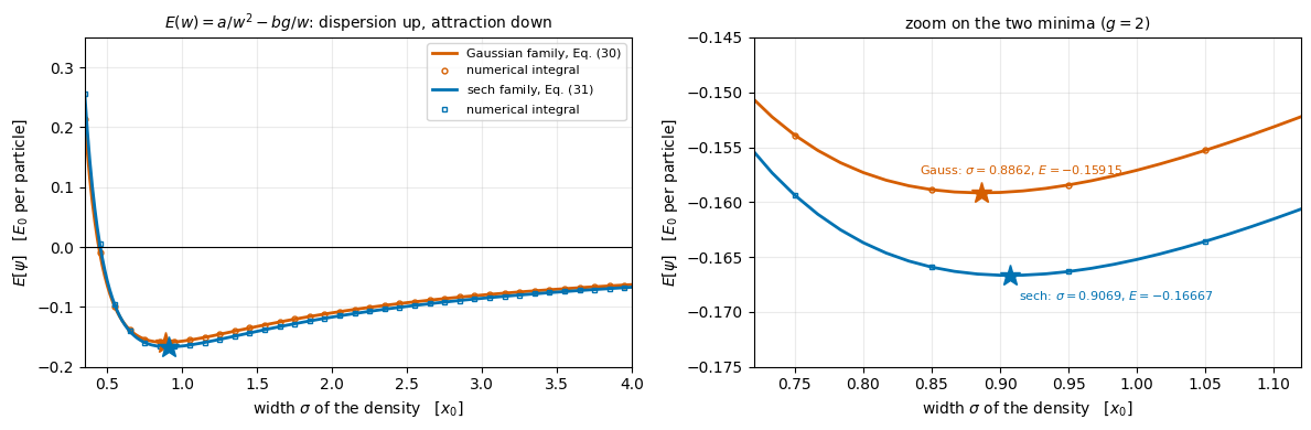
11.5 Outlook: two solitons

The same propagator can launch two solitons at each other. They pass straight through and emerge with their shapes intact and only a shift in position and phase, the signature of integrability. What happens during the overlap depends on the relative phase, which Ref. [48] measured directly.

---

Marcin Płodzień, PhD

Citation: M. Płodzień, Quantum Many-Body Simulation: from a single spin to quantum machine learning (2026), https://marcinplodzien.github.io/quantum-many-body-simulation/