Entanglement of a Parametric Two-Qubit State

Mathematical Foundations, numerical solution.

Entanglement of a Parametric Two-Qubit State

---

Background

When two systems share a joint pure state, a measurement on one can be correlated with the other in ways no shared classical variable could reproduce. That excess correlation is entanglement, and in the pure-state case it has a clean signature. An observer holding only one of the two subsystems cannot see the global state and instead works with the reduced density matrix obtained by tracing out the partner. For a product state this reduced state is itself pure and the subsystem carries definite information of its own. Once the parts are entangled the reduced state turns mixed, and the more mixed it becomes, the more entanglement the pair holds.

Mixedness needs a number to track it. One choice is the purity, which equals one for a pure state and drops as the state spreads over more eigenvalues. Another is the von Neumann entropy, which is zero for a pure state and climbs toward its maximum as those eigenvalues even out. For a pair of qubits the reduced state has only two eigenvalues, so a single weight fixes both quantities at once.

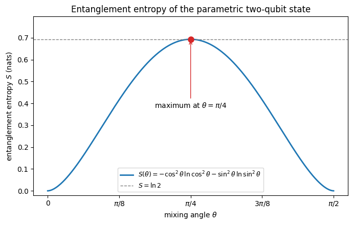
The family \(\cos\theta\,|00\rangle + \sin\theta\,|11\rangle\) is already written in its Schmidt form, meaning the entanglement is laid bare by the two coefficients with no further diagonalization needed. The reduced density matrix is diagonal with eigenvalues \(\cos^2\theta\) and \(\sin^2\theta\), and its von Neumann entropy is the binary entropy of those weights, a single curve in the mixing angle. The ends \(\theta = 0\) and \(\theta = \pi/2\) put all the weight on one term and give product states, while \(\theta = \pi/4\) balances the two and produces a Bell state whose reduced density matrix is maximally mixed.

This exercise traces out one qubit, computes the purity and the von Neumann entropy across the family, and locates the separable and maximally entangled points.

Mathematical background

The entanglement of a pure bipartite state is read from the Schmidt decomposition

\[ |\psi\rangle = \sum_i \sqrt{p_i}\,|i\rangle_A\,|i\rangle_B , \]

whose coefficients \(\sqrt{p_i}\) are the singular values of the coefficient matrix and whose squares \(p_i\) are the eigenvalues of the reduced density matrix \(\rho_A = \mathrm{Tr}_B|\psi\rangle\langle\psi|\). The state is a product exactly when one \(p_i = 1\), and maximally entangled when the \(p_i\) are all equal. The entanglement entropy

\[ S(\rho_A) = -\sum_i p_i \log p_i \]

interpolates between these limits. For two qubits the reduced state is \(2\times 2\), so a single Schmidt angle controls the entanglement, and it can equally be tracked by the purity \(\mathrm{Tr}\,\rho_A^2 = \sum_i p_i^2\) or the concurrence. As a tunable coupling in the state is varied, the Schmidt weights shift continuously and the entropy traces out how strongly the two qubits are correlated along the path.

Exercise

Consider the parametric two-qubit state:

\[ |\psi(\theta)\rangle = \cos\theta\,|00\rangle + \sin\theta\,|11\rangle. \]

(a) Compute the reduced density matrix \(\rho_A = \mathrm{Tr}_B(|\psi\rangle\langle\psi|)\).

(b) Compute the purity \(\gamma = \mathrm{Tr}(\rho_A^2)\) and the von Neumann entropy \(S = -\mathrm{Tr}(\rho_A \ln \rho_A)\) as functions of \(\theta\).

(c) Show the state is maximally entangled at \(\theta = \pi/4\) and separable at \(\theta = 0, \pi/2\).

Solution

Part (a): Reduced density matrix

The full density matrix is:

\[ |\psi\rangle\langle\psi| = \cos^2\!\theta\,|00\rangle\langle 00| + \sin^2\!\theta\,|11\rangle\langle 11| + \cos\theta\sin\theta\bigl(|00\rangle\langle 11| + |11\rangle\langle 00|\bigr). \]

Tracing over subsystem \(B\): the partial trace acts on the second tensor factor. The diagonal terms survive since \(\langle 0|0\rangle = \langle 1|1\rangle = 1\). The off-diagonal terms vanish because \(\langle 0|1\rangle = 0\):

\[ \mathrm{Tr}_B(|00\rangle\langle 11|) = |0\rangle\langle 1| \cdot \underbrace{\langle 1|0\rangle}_{=\,0} = 0. \]

Therefore:

\[ \boxed{\rho_A = \cos^2\!\theta\,|0\rangle\langle 0| + \sin^2\!\theta\,|1\rangle\langle 1| = \begin{pmatrix} \cos^2\!\theta & 0 \\ 0 & \sin^2\!\theta \end{pmatrix}.} \]

The reduced state is diagonal in the computational basis, with eigenvalues \(\lambda_0 = \cos^2\!\theta\) and \(\lambda_1 = \sin^2\!\theta\).

Part (b): Purity and entropy

Purity:

\[ \gamma = \mathrm{Tr}(\rho_A^2) = \cos^4\!\theta + \sin^4\!\theta. \]

Using the identity \(\cos^4\!\theta + \sin^4\!\theta = 1 - 2\cos^2\!\theta\sin^2\!\theta = 1 - \frac{1}{2}\sin^2\!(2\theta)\):

\[ \gamma = 1 - \frac{1}{2}\sin^2(2\theta). \]

Von Neumann entropy:

\[ S = -\cos^2\!\theta\,\ln(\cos^2\!\theta) - \sin^2\!\theta\,\ln(\sin^2\!\theta). \]

This is the binary entropy function \(h(\cos^2\!\theta)\).

Part (c): Extremal cases

\(\theta = \pi/4\) (maximally entangled): \(\cos^2(\pi/4) = \sin^2(\pi/4) = 1/2\).

\[ \rho_A = \frac{I}{2}, \qquad \gamma = \frac{1}{2}, \qquad S = \ln 2. \]

The reduced state is maximally mixed, one bit of entanglement. The state is the Bell state \((|00\rangle + |11\rangle)/\sqrt{2}\).

\(\theta = 0\) or \(\pi/2\) (separable): The state is \(|00\rangle\) or \(|11\rangle\), a product state.

\[ \rho_A = |0\rangle\langle 0| \text{ or } |1\rangle\langle 1|, \qquad \gamma = 1, \qquad S = 0. \]

Zero entanglement. The purity is maximal (\(\gamma = 1\)), confirming the reduced state is pure, the hallmark of a product state.

---

Symbolic Verification (SymPy)

Code

import sympy as sp

t = sp.Symbol('theta', real=True, positive=True)

lam0 = sp.cos(t)**2
lam1 = sp.sin(t)**2

# Purity
gamma = sp.trigsimp(lam0**2 + lam1**2)
print(f"γ = {gamma}")

# Entropy
S = sp.simplify(-lam0*sp.log(lam0) - lam1*sp.log(lam1))
print(f"S = {S}")

# At theta = pi/4
gamma_max_ent = gamma.subs(t, sp.pi/4)
S_max_ent = S.subs(t, sp.pi/4)
print(f"θ=π/4: γ = {gamma_max_ent}, S = {sp.simplify(S_max_ent)}")
assert gamma_max_ent == sp.Rational(1,2)
assert sp.simplify(S_max_ent - sp.log(2)) == 0

γ = sin(theta)**4 + cos(theta)**4
S = -log(sin(theta)**2)*sin(theta)**2 - log(cos(theta)**2)*cos(theta)**2
θ=π/4: γ = 1/2, S = log(2)

---

Numerical Verification

Code

import numpy as np

thetas = np.linspace(0, np.pi/2, 9)
print(f"{'θ/π':>8s}  {'γ':>8s}  {'S':>8s}  {'S/ln2':>8s}")
print(f"{'─'*8:>8s}  {'─'*8:>8s}  {'─'*8:>8s}  {'─'*8:>8s}")

for theta in thetas:
    c2 = np.cos(theta)**2
    s2 = np.sin(theta)**2
    gamma = c2**2 + s2**2
    eigs = np.array([c2, s2])
    eigs_pos = eigs[eigs > 1e-15]
    S = -np.sum(eigs_pos * np.log(eigs_pos))
    print(f"{theta/np.pi:8.4f}  {gamma:8.4f}  {S:8.4f}  {S/np.log(2):8.4f}")

print("\nMaximal entanglement at θ = π/4 (S = ln2).")

     θ/π         γ         S     S/ln2
────────  ────────  ────────  ────────
  0.0000    1.0000   -0.0000   -0.0000
  0.0625    0.9268    0.1617    0.2333
  0.1250    0.7500    0.4165    0.6009
  0.1875    0.5732    0.6180    0.8916
  0.2500    0.5000    0.6931    1.0000
  0.3125    0.5732    0.6180    0.8916
  0.3750    0.7500    0.4165    0.6009
  0.4375    0.9268    0.1617    0.2333
  0.5000    1.0000   -0.0000   -0.0000

Maximal entanglement at θ = π/4 (S = ln2).

---

Entanglement Entropy versus the Mixing Angle

Code

%matplotlib inline
import numpy as np
import matplotlib.pyplot as plt

theta = np.linspace(0, np.pi/2, 400)
c2 = np.cos(theta)**2
s2 = np.sin(theta)**2

# Von Neumann entropy of the reduced state (natural log)
with np.errstate(divide='ignore', invalid='ignore'):
    terms = -np.where(c2 > 0, c2*np.log(c2), 0.0) - np.where(s2 > 0, s2*np.log(s2), 0.0)
S = terms

fig, ax = plt.subplots(figsize=(7, 4.5))
ax.plot(theta, S, color='C0', lw=2, label=r'$S(\theta) = -\cos^2\theta\,\ln\cos^2\theta - \sin^2\theta\,\ln\sin^2\theta$')
ax.axhline(np.log(2), color='gray', ls='--', lw=1, label=r'$S = \ln 2$')
ax.plot(np.pi/4, np.log(2), 'o', color='C3', ms=8, zorder=5)
ax.annotate(r'maximum at $\theta=\pi/4$', xy=(np.pi/4, np.log(2)),
            xytext=(np.pi/4, np.log(2)*0.55), ha='center',
            arrowprops=dict(arrowstyle='->', color='C3'))

ax.set_xlabel(r'mixing angle $\theta$')
ax.set_ylabel(r'entanglement entropy $S$ (nats)')
ax.set_title('Entanglement entropy of the parametric two-qubit state')
ax.set_xticks([0, np.pi/8, np.pi/4, 3*np.pi/8, np.pi/2])
ax.set_xticklabels(['0', r'$\pi/8$', r'$\pi/4$', r'$3\pi/8$', r'$\pi/2$'])
ax.set_ylim(-0.02, np.log(2)*1.15)
ax.legend(loc='lower center', fontsize=9)
plt.tight_layout()
plt.show()

---

Takeaway

The entropy follows a binary entropy curve in the mixing angle, rising to its maximum \(S = \ln 2\) at \(\theta = \pi/4\) where the reduced state is maximally mixed. The endpoints \(\theta = 0, \pi/2\) are product states with zero entanglement; the peak is the Bell state carrying one bit.

References

• Page, Average entropy of a subsystem, Physical Review Letters (1993).
• Horodecki et al., Quantum entanglement, Reviews of Modern Physics (2009).
• Nielsen and Chuang, Quantum Computation and Quantum Information, Cambridge University Press (2010).
• Płodzień, Information Scrambling, Quantum Chaos, and Haar-Random States, lecture notes (2025). arXiv:2511.14397