Eigenphase Repulsion in the CUE

Random Matrix Theory, numerical solution.

Eigenphase Repulsion in the \(2 \times 2\) CUE

Background

The eigenvalues of a Haar-random unitary all sit on the unit circle, each one a pure phase \(e^{i\theta}\). Their angles are not thrown down independently, because the joint distribution of the phases contains the squared Vandermonde factor \(\prod_{j<k}|e^{i\theta_j}-e^{i\theta_k}|^2\). This factor shrinks toward zero whenever two phases approach each other, so configurations with nearly coincident eigenvalues are strongly disfavored. The resulting ensemble is the Circular Unitary Ensemble, the unitary-group counterpart of the Gaussian models for Hermitian matrices.

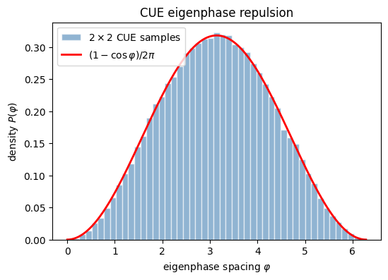
For two eigenvalues the calculation can be carried all the way through. Reducing the Vandermonde factor to the single gap variable gives the spacing density \(P(\varphi) = (1-\cos\varphi)/(2\pi)\), where \(\varphi\) is the angular separation of the two phases. The density is largest when the phases sit diametrically opposite on the circle and falls off as they come together.

Near zero spacing the density vanishes like \(\varphi^2\), a quadratic repulsion that marks the \(\beta = 2\) unitary symmetry class and is stronger than the linear repulsion seen in the time-reversal-symmetric case. The same quadratic repulsion turns up far beyond random matrices, in the spectra of heavy nuclei and even in the spacing of the zeros of the Riemann zeta function, where the same statistics appear.

The notebook reduces the Vandermonde factor to the spacing variable and compares the normalized density against phases sampled from random \(U(2)\) matrices.

Mathematical background

The circular unitary ensemble is \(U(D)\) under the Haar measure, and its eigenvalues are pure phases \(e^{i\theta_j}\) on the unit circle. Integrating out the eigenvectors leaves the Weyl joint density of the eigenphases,

\[ P(\theta_1,\dots,\theta_D) \propto \prod_{j<k}\big|e^{i\theta_j} - e^{i\theta_k}\big|^2 , \]

the circular counterpart of the Vandermonde-squared weight of the \(\beta = 2\) Gaussian ensembles. Since \(|e^{i\theta_j} - e^{i\theta_k}|^2 = 2 - 2\cos(\theta_j-\theta_k)\) vanishes quadratically as two phases approach, the eigenphases repel with the same exponent as the GUE. The mean density is uniform at \(D/2\pi\), and the connected pair correlation has the sine-kernel form \(-\big(\sin(\pi r)/\pi r\big)^2\) in the unfolded spacing \(r\), identical to the GUE bulk. Unitary and Hermitian chaotic spectra therefore share their local statistics, which is why the CUE is the natural random-matrix model for Floquet and scattering systems, where the evolution operator rather than a Hamiltonian is the object of interest.

Exercise

A \(2 \times 2\) CUE matrix (Haar-random \(U \in U(2)\)) has eigenvalues \(e^{i\theta_1}, e^{i\theta_2}\) with joint density proportional to the Vandermonde squared:

\[ P(\theta_1, \theta_2) \propto |e^{i\theta_1} - e^{i\theta_2}|^2. \]

(a) Show \(|e^{i\theta_1} - e^{i\theta_2}|^2 = 2 - 2\cos(\theta_1 - \theta_2)\).

(b) With \(\varphi = \theta_1 - \theta_2\), show the spacing density is \(P(\varphi) = (1 - \cos\varphi)/(2\pi)\).

(c) Verify \(P(0) = 0\) (level repulsion) and find the most probable spacing.

Solution

Part (a): Algebraic identity

Expand the modulus squared:

\[ |e^{i\theta_1} - e^{i\theta_2}|^2 = (e^{i\theta_1} - e^{i\theta_2})(e^{-i\theta_1} - e^{-i\theta_2}) \]

\[ = 1 - e^{i(\theta_1 - \theta_2)} - e^{-i(\theta_1 - \theta_2)} + 1 = 2 - 2\cos(\theta_1 - \theta_2). \quad \checkmark \]

Key feature: the expression depends only on the spacing \(\varphi = \theta_1 - \theta_2\), not on the individual phases.

Part (b): Marginal spacing density

Change variables to the spacing \(\varphi = \theta_1 - \theta_2\) and the center of mass \(\Theta = (\theta_1 + \theta_2)/2\).

The joint density is \(P(\varphi, \Theta) \propto 2 - 2\cos\varphi\). Integrating over the center of mass \(\Theta \in [0, 2\pi)\) gives a factor \(2\pi\).

The normalization constant is

\[ Z = \int_0^{2\pi} (2 - 2\cos\varphi)\, d\varphi = [2\varphi - 2\sin\varphi]_0^{2\pi} = 4\pi. \]

Therefore the normalized spacing density is

\[ \boxed{P(\varphi) = \frac{1 - \cos\varphi}{2\pi}.} \]

Part (c): Level repulsion and most probable spacing

Level repulsion: At \(\varphi = 0\):

\[ P(0) = \frac{1 - 1}{2\pi} = 0. \]

Eigenphases cannot coincide, there is a strict vanishing of the density at zero spacing. Near \(\varphi = 0\), \(P(\varphi) \approx \varphi^2/(4\pi)\): the repulsion is quadratic (\(\beta = 2\) for the CUE).

Most probable spacing: Maximize \(P(\varphi) = (1 - \cos\varphi)/(2\pi)\):

\[ \frac{dP}{d\varphi} = \frac{\sin\varphi}{2\pi} = 0 \quad \Rightarrow \quad \varphi = \pi. \]

Eigenphases prefer to sit diametrically opposite on the unit circle, the maximally separated configuration. This is the most basic manifestation of spectral rigidity.

Symbolic Verification (SymPy)

Code

import sympy as sp

t1, t2, phi = sp.symbols('theta_1 theta_2 phi', real=True)

# Part (a)
expr = sp.expand(sp.Abs(sp.exp(sp.I*t1) - sp.exp(sp.I*t2))**2)
expr_simplified = sp.trigsimp(sp.expand_complex(expr))
print(f"|e^{{iθ₁}} − e^{{iθ₂}}|² = {expr_simplified}")

# Part (b): normalization
Z = sp.integrate(2 - 2*sp.cos(phi), (phi, 0, 2*sp.pi))
print(f"Z = ∫(2−2cosφ)dφ = {Z}")
P = (1 - sp.cos(phi)) / (2*sp.pi)
norm = sp.integrate(P, (phi, 0, 2*sp.pi))
print(f"∫ P(φ) dφ = {norm}")
assert norm == 1

|e^{iθ₁} − e^{iθ₂}|² = 2 - 2*cos(theta_1 - theta_2)
Z = ∫(2−2cosφ)dφ = 4*pi
∫ P(φ) dφ = 1

Numerical Verification

Code

import numpy as np
from scipy.stats import unitary_group

np.random.seed(42)

# Sample eigenphase spacings from Haar-random U(2).
# The spacing φ = θ₁ − θ₂ is the difference of the two eigenphases
# taken on the circle (mod 2π).  Do NOT sort the phases first: sorting
# the principal values in (−π, π] yields a *linear* gap whose
# distribution differs from the circular spacing density.
n_samples = 50000
spacings = []
for _ in range(n_samples):
    U = unitary_group.rvs(2)
    phases = np.angle(np.linalg.eigvals(U))
    phi = (phases[1] - phases[0]) % (2*np.pi)
    spacings.append(phi)

spacings = np.array(spacings)

# Histogram vs analytical P(φ)
bins = np.linspace(0, 2*np.pi, 50)
centers = (bins[:-1] + bins[1:]) / 2
hist, _ = np.histogram(spacings, bins=bins, density=True)
P_theory = (1 - np.cos(centers)) / (2*np.pi)

residual = np.max(np.abs(hist - P_theory))
print(f"Max |histogram − P(φ)| = {residual:.4f}")
assert residual < 0.02

# Check P(0) → 0: fraction of spacings < 0.1
frac_small = np.mean(spacings < 0.1)
print(f"Fraction with φ < 0.1: {frac_small:.4f} (level repulsion)")

# Most probable spacing
mode = centers[np.argmax(hist)]
print(f"Most probable spacing: {mode:.2f} (expected π = {np.pi:.2f})")
print("\nLevel repulsion confirmed.")

Max |histogram − P(φ)| = 0.0128
Fraction with φ < 0.1: 0.0000 (level repulsion)
Most probable spacing: 3.14 (expected π = 3.14)

Level repulsion confirmed.

Code

%matplotlib inline
import matplotlib.pyplot as plt

phi_grid = np.linspace(0, 2*np.pi, 400)
P_grid = (1 - np.cos(phi_grid)) / (2*np.pi)

fig, ax = plt.subplots(figsize=(6, 4))
ax.hist(spacings, bins=bins, density=True, alpha=0.6,
        color='steelblue', edgecolor='white', label='$2\\times 2$ CUE samples')
ax.plot(phi_grid, P_grid, 'r-', lw=2,
        label=r'$(1-\cos\varphi)/2\pi$')
ax.set_xlabel(r'eigenphase spacing $\varphi$')
ax.set_ylabel(r'density $P(\varphi)$')
ax.set_title('CUE eigenphase repulsion')
ax.legend()
plt.show()

Takeaway

The \(2 \times 2\) CUE eigenphase spacing follows \(P(\varphi) = (1 - \cos\varphi)/(2\pi)\), vanishing at \(\varphi = 0\) and peaking at \(\varphi = \pi\). The histogram shows level repulsion at small spacing.

Connections

The circular unitary ensemble is precisely the Haar measure on the unitary group, so the eigenphase repulsion here is the unitary version of the GOE level spacing for Hamiltonians. It is the same measure whose low moments are evaluated throughout the Weingarten notebooks. The statistics you see in the eigenphases and the averages you compute there come from one distribution.

References

Dyson, Statistical theory of the energy levels of complex systems. I, Journal of Mathematical Physics (1962).
Mezzadri, How to generate random matrices from the classical compact groups, Notices of the American Mathematical Society (2007).
Mehta, Random matrices, Academic Press (2004).
Płodzień, Information Scrambling, Quantum Chaos, and Haar-Random States, lecture notes (2025). arXiv:2511.14397