Krylov Complexity from the Geometric Distribution

Quantum Dynamics & Chaos, numerical solution.

Krylov Complexity from the Geometric Distribution

Background

As an operator evolves in time it spreads through the space of operators, and Krylov complexity is one way to quantify how far it has gone. The idea starts with the Lanczos algorithm, which builds an orthonormal chain of operators by repeatedly taking commutators with the Hamiltonian. Along this chain the evolution looks like a particle hopping between neighboring sites, with hopping amplitudes called the Lanczos coefficients. The complexity is the average position of the operator on the chain, small when it remains near its starting point and large once it has migrated far down.

The motion is governed entirely by how the Lanczos coefficients grow with chain index. The notebook treats the case where they grow linearly, the amplitude at site \(n\) proportional to \(n\). This linear growth is the signature of the most strongly chaotic systems, and it lets the hopping problem be solved in closed form. The amplitude profile along the chain becomes a geometric distribution whose width spreads in time.

Carrying out the sums, the complexity works out to \(C_K(t) = \sinh^2(\alpha t)\), where \(\alpha\) sets the rate. At late times this grows like \(e^{2\alpha t}\), an exponential spreading of the operator down the chain. The growth rate plays the role of a Lyapunov exponent for operator dynamics and bounds the exponent that governs the related out-of-time-order correlator, which is why Krylov complexity works as a chaos diagnostic that needs no averaging over an ensemble.

The linear-coefficient assumption describes the maximally chaotic limit, and generic systems depart from it once the chain index grows large. The notebook derives the closed form \(C_K(t) = \sinh^2(\alpha t)\) from the geometric distribution and confirms it, together with the variance of the position, by summing the chain numerically.

Mathematical background

Operator growth can be recast as a single-particle hopping problem through the Lanczos algorithm. Starting from an operator \(\mathcal{O}\) and the Liouvillian \(\mathcal{L} = [H, \cdot]\), repeated application of \(\mathcal{L}\) with Gram-Schmidt orthogonalization builds the Krylov basis \(\{\mathcal{O}_n\}\), in which \(\mathcal{L}\) is tridiagonal,

\[ \mathcal{L}\,\mathcal{O}_n = b_{n+1}\,\mathcal{O}_{n+1} + b_n\,\mathcal{O}_{n-1}. \]

The Heisenberg evolution then maps onto an amplitude \(\varphi_n(t)\) on a semi-infinite chain with hopping amplitudes \(b_n\), the Lanczos coefficients, and the Krylov complexity is the mean position on that chain,

\[ \mathcal{C}_K(t) = \sum_n n\,|\varphi_n(t)|^2 . \]

The rate at which the \(b_n\) grow controls how fast the operator spreads. The universal operator-growth hypothesis holds that for chaotic systems the \(b_n\) grow as fast as locality allows, asymptotically linearly with \(b_n \sim \alpha n\), and a linear ramp of hopping amplitudes drives exponential growth of the position, \(\mathcal{C}_K(t) \sim e^{2\alpha t}\). The slope \(\alpha\) upper-bounds the Lyapunov exponent of the out-of-time-ordered correlator, so Krylov complexity is a basis-independent diagnostic of scrambling that needs no choice of probe operator.

Motivation

Krylov complexity \(C_K(t)\) measures how far an operator has spread in the Krylov basis, an orthonormal basis generated by repeated commutation with the Hamiltonian (the Lanczos algorithm). When the Lanczos coefficients grow linearly (\(b_n = \alpha n\)), the Krylov amplitudes take a closed form: a geometric distribution on the Krylov chain. The resulting complexity \(C_K(t) = \sinh^2(\alpha t)\) grows exponentially, the operator-growth analogue of a Lyapunov exponent.

Preliminaries / Toolbox

Krylov basis: Given an initial operator \(\mathcal{O}_0\) and Hamiltonian \(H\), the Lanczos algorithm constructs an orthonormal basis \(\{\mathcal{O}_n\}\) for the operator Hilbert space such that the Liouvillian \(\mathcal{L} = [H, \cdot]\) acts tridiagonally:

\[ \mathcal{L}|\mathcal{O}_n) = b_{n+1}|\mathcal{O}_{n+1}) + b_n|\mathcal{O}_{n-1}). \]

The Lanczos coefficients \(\{b_n\}\) encode the growth rate. The operator at time \(t\) is \(\mathcal{O}(t) = \sum_n \varphi_n(t) \mathcal{O}_n\).

Krylov complexity: \(C_K(t) = \sum_n n\, |\varphi_n(t)|^2\), the average position on the Krylov chain.

Geometric series: For \(|r| < 1\): \(\sum_{n=0}^\infty r^n = \frac{1}{1-r}\), \(\sum_{n=0}^\infty n r^n = \frac{r}{(1-r)^2}\).

Hyperbolic identities: \(\tanh^2 x + \mathrm{sech}^2 x = 1\), \(\sinh^2 x = \tanh^2 x \cdot \cosh^2 x\).

Exercise

When \(b_n = \alpha n\), the Krylov amplitudes are \(\varphi_n(t) = \tau^n / c\) with \(\tau(t) = \tanh(\alpha t)\), \(c(t) = \cosh(\alpha t)\).

(a) Verify \(\sum_n |\varphi_n|^2 = 1\).

(b) Compute \(C_K(t) = \sum_n n |\varphi_n|^2\) and show \(C_K(t) = \sinh^2(\alpha t)\).

(c) Compute \(\mathrm{Var}(n)\).

Solution

Part (a): Normalization

The probability distribution on the Krylov chain is:

\[ p_n = |\varphi_n|^2 = \frac{\tau^{2n}}{c^2} = (1 - \tau^2)\, \tau^{2n}, \]

where we used \(1/c^2 = 1/\cosh^2 = 1 - \tanh^2 = 1 - \tau^2\). This is a geometric distribution with ratio \(r = \tau^2 < 1\):

\[ \sum_{n=0}^\infty p_n = (1 - \tau^2) \sum_{n=0}^\infty \tau^{2n} = (1-\tau^2) \cdot \frac{1}{1-\tau^2} = 1. \quad \checkmark \]

Part (b): Krylov complexity

\[ C_K = \sum_n n\, p_n = (1-\tau^2) \sum_n n\, \tau^{2n} = (1-\tau^2) \cdot \frac{\tau^2}{(1-\tau^2)^2} = \frac{\tau^2}{1-\tau^2}. \]

Substituting \(\tau = \tanh(\alpha t)\) and \(1 - \tanh^2 = \mathrm{sech}^2 = 1/\cosh^2\):

\[ C_K = \tanh^2(\alpha t) \cdot \cosh^2(\alpha t) = \sinh^2(\alpha t). \]

\[ \boxed{C_K(t) = \sinh^2(\alpha t) \approx \tfrac{1}{4}e^{2\alpha t} \quad (t \gg 1/\alpha).} \]

This exponential growth at rate \(2\alpha\) is the operator-growth Lyapunov exponent.

Part (c): Variance

\[ \langle n^2 \rangle = (1-\tau^2)\sum_n n^2 \tau^{2n} = (1-\tau^2) \cdot \frac{\tau^2(1+\tau^2)}{(1-\tau^2)^3} = \frac{\tau^2(1+\tau^2)}{(1-\tau^2)^2}. \]

\[ \mathrm{Var}(n) = \langle n^2 \rangle - \langle n \rangle^2 = \frac{\tau^2(1+\tau^2)}{(1-\tau^2)^2} - \frac{\tau^4}{(1-\tau^2)^2} = \frac{\tau^2}{(1-\tau^2)^2}. \]

In hyperbolic functions: \(\mathrm{Var} = \sinh^2 \cdot \cosh^2 = \frac{1}{4}\sinh^2(2\alpha t)\).

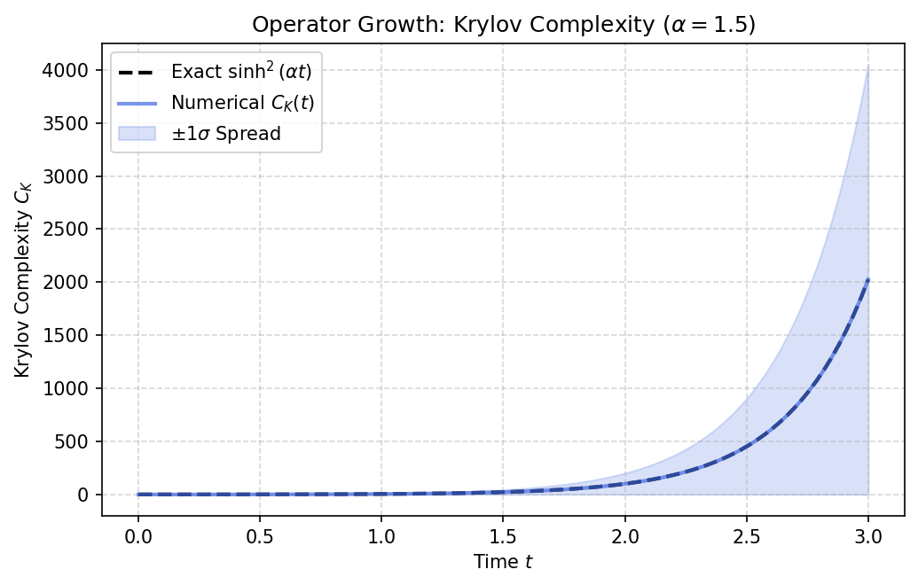
The standard deviation \(\sigma \sim e^{2\alpha t}\) grows at the same exponential rate as the mean, so the wavepacket keeps a fixed relative width while its position runs exponentially down the Krylov chain.

Symbolic Verification (SymPy)

Code

import sympy as sp

alpha, t = sp.symbols('alpha t', positive=True)
n = sp.Symbol('n', nonneg=True, integer=True)

# Geometric distribution: p_n = (1-tanh^2(alpha*t)) * tanh^{2n}(alpha*t)
tau = sp.tanh(alpha * t)
p_n = (1 - tau**2) * tau**(2*n)

# Krylov complexity C_K = sum_n n * p_n = sinh^2(alpha*t)
# Verify: sum of geometric series
# C_K = (1-tau^2) * tau^2 / (1-tau^2)^2 = tau^2/(1-tau^2) = sinh^2
C_K_formula = tau**2 / (1 - tau**2)
C_K_expected = sp.sinh(alpha * t)**2
diff = sp.simplify(C_K_formula - C_K_expected)
print(f'C_K from geometric sum = {C_K_formula}')
print(f'sinh^2(alpha*t) = {C_K_expected}')
print(f'Difference = {diff}')
assert diff == 0
print('Verified: C_K(t) = sinh^2(alpha*t)')

C_K from geometric sum = tanh(alpha*t)**2/(1 - tanh(alpha*t)**2)
sinh^2(alpha*t) = sinh(alpha*t)**2
Difference = 0
Verified: C_K(t) = sinh^2(alpha*t)

Numerical Verification

Code

import numpy as np

alpha = 1.5
n_max = 100000  # truncation of the infinite Krylov sum (needs many terms at large t)
ns = np.arange(n_max)

print(f"α = {alpha}")
print(f"{'t':>5s}  {'C_K (sum)':>12s}  {'sinh²(αt)':>12s}  {'Var(sum)':>12s}  {'Var(pred)':>12s}")
print(f"{'─'*5:>5s}  {'─'*12:>12s}  {'─'*12:>12s}  {'─'*12:>12s}  {'─'*12:>12s}")

for t in [0.1, 0.5, 1.0, 1.5, 2.0, 3.0]:
    tau = np.tanh(alpha*t)
    p = (1 - tau**2) * tau**(2*ns)

    norm = np.sum(p)
    CK_sum = np.sum(ns * p)
    CK_pred = np.sinh(alpha*t)**2
    var_sum = np.sum(ns**2 * p) - CK_sum**2
    var_pred = tau**2 / (1 - tau**2)**2

    print(f"{t:5.1f}  {CK_sum:12.4f}  {CK_pred:12.4f}  {var_sum:12.4f}  {var_pred:12.4f}")
    assert abs(norm - 1) < 1e-4
    assert abs(CK_sum - CK_pred) / max(CK_pred, 1) < 0.01

print("\nKrylov complexity = sinh²(αt) confirmed.")

α = 1.5
    t     C_K (sum)     sinh²(αt)      Var(sum)     Var(pred)
─────  ────────────  ────────────  ────────────  ────────────
  0.1        0.0227        0.0227        0.0232        0.0232
  0.5        0.6762        0.6762        1.1335        1.1335
  1.0        4.5338        4.5338       25.0895       25.0895
  1.5       22.0071       22.0071      506.3178      506.3178
  2.0      100.3578      100.3578    10172.0495    10172.0495
  3.0     2025.2710     2025.2710  4103747.9461  4103747.9461

Krylov complexity = sinh²(αt) confirmed.

Visual Pedagogical Proof

Code

import matplotlib.pyplot as plt

alpha = 1.5
n_max = 100000
ns_arr = np.arange(n_max)
times_k = np.linspace(0, 3, 100)

CK_vals = []
var_vals = []
for t_k in times_k:
    tau = np.tanh(alpha*t_k)
    p = (1 - tau**2) * tau**(2*ns_arr)
    CK_vals.append(np.sum(ns_arr * p))
    var_vals.append(np.sum(ns_arr**2 * p) - np.sum(ns_arr * p)**2)

CK_exact = np.sinh(alpha*times_k)**2

plt.rcParams['figure.dpi'] = 150
plt.figure(figsize=(7, 4.5))
plt.plot(times_k, CK_exact, 'k--', linewidth=2, label=r'Exact $\sinh^2(\alpha t)$')
plt.plot(times_k, CK_vals, 'royalblue', linewidth=2, alpha=0.7, label=r'Numerical $C_K(t)$')
plt.fill_between(times_k, np.maximum(0, np.array(CK_vals) - np.sqrt(var_vals)),
                 np.array(CK_vals) + np.sqrt(var_vals), color='royalblue', alpha=0.2, label=r'$\pm 1\sigma$ Spread')

plt.xlabel(r"Time $t$")
plt.ylabel(r"Krylov Complexity $C_K$")
plt.title(r"Operator Growth: Krylov Complexity ($\alpha=1.5$)")
plt.legend(loc='upper left')
plt.grid(True, ls="--", alpha=0.5)
plt.tight_layout()
plt.show()

Takeaway

Linearly growing Lanczos coefficients produce a geometric distribution on the Krylov chain and complexity \(C_K(t) = \sinh^2(\alpha t)\). Mean and standard deviation both scale as \(e^{2\alpha t}\), so the operator’s position on the chain grows exponentially at rate \(2\alpha\), the operator-growth Lyapunov exponent.

References

Parker et al., A Universal Operator Growth Hypothesis, Physical Review X (2019).
Lanczos, An iteration method for the solution of the eigenvalue problem of linear differential and integral operators, Journal of Research of the National Bureau of Standards (1950).
Balasubramanian et al., Quantum chaos and the complexity of spread of states, Physical Review D (2022).
Viswanath and Müller, The Recursion Method: Application to Many-Body Dynamics, Springer (1994).
Płodzień, Information Scrambling, Quantum Chaos, and Haar-Random States, lecture notes (2025). arXiv:2511.14397