Quantum Extreme Learning Machines and the POVM Picture
This exercise develops the complete theory of why deep quantum circuits destroy the utility of Quantum Extreme Learning Machines. We begin with the physical picture, formalize the POVM structure, and then prove three escalating results about signal death under Haar scrambling.
Background
A quantum extreme learning machine keeps the training almost trivial and lets the physics do the hard part. Data is encoded into a fixed random circuit that is never optimized, and only a linear readout on the measured probabilities is fit afterward. The quantum dynamics supply whatever nonlinearity the model needs, and the learning step stays a plain linear regression. The circuit acts on the input together with an auxiliary reservoir register, and tracing the reservoir out recasts each readout feature as a Born probability on the input alone, \(f_b(x) = \mathrm{Tr}(M_b\,\rho_{\mathrm{in}}(x))\), where \(M_b\) is an effective measurement operator. What matters is how much of the input still shows through these features once the circuit has mixed everything together.
Under a random reservoir the averaging washes the operators out. The mean effective measurement is \(\mathbb{E}[M_b] = I_{\mathrm{in}}/D\), a flat operator proportional to the identity, so every feature averages to \(1/D\) regardless of which input was encoded. The mean therefore carries no information at all about \(x\), and whatever the model can learn must live in the fluctuations around it.
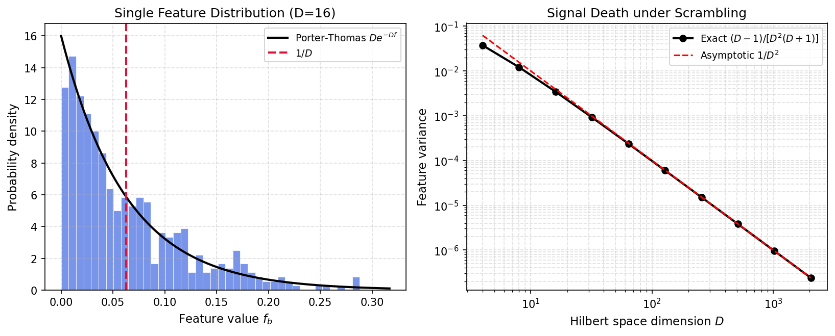
Those fluctuations are small. The variance of a feature is of order \(1/D^2\) with \(D = 2^N\), so the input-dependent part of \(f_b(x)\) is a faint ripple riding on a uniform \(1/D\) background. The signal is present, but it is exponentially fainter than the constant it sits on.
This sets a hard floor on measurement. Resolving the \(1/D\) ripple against shot noise takes more than \(D = 2^N\) measurements per feature before any input dependence becomes visible. A reservoir that works has to sit close to the onset of scrambling, deep enough that the effective measurements reach across a wide subspace yet shallow enough to keep their dependence on the input above the sampling floor.
1. The Physical Setup
Consider a quantum device with two registers:
An input register of \(N_{\mathrm{in}}\) qubits, encoding classical data \(x\) via a state \(\rho_{\mathrm{in}}(x)\).
A reservoir register of \(N_{\mathrm{res}}\) qubits, initialized in the fiducial state \(|0\rangle^{\otimes N_{\mathrm{res}}}\).
The total Hilbert space dimension is \(D = 2^{N_{\mathrm{in}} + N_{\mathrm{res}}}\). A fixed (but random) unitary \(U\) acts on the joint system, and features are extracted by measuring in the computational basis:
The \(D\) real numbers \(\{f_b(x)\}_{b=0}^{D-1}\) form the feature vector that a classical linear model is trained on. The central question is: how much information about \(x\) survives in these features when \(U\) is a deep, chaotic circuit?
2. The POVM Perspective: Naimark Dilation in Reverse
A powerful way to understand the QELM is to recognize that the entire pipeline, tensoring with the reservoir, applying \(U\), and projecting onto \(|b\rangle\), defines an effective measurement on the input register alone.
Tracing over the reservoir degrees of freedom, each computational basis outcome \(b\) corresponds to a POVM element acting on the input space \(\mathcal{H}_{\mathrm{in}}\):
These satisfy the POVM axioms: 1. Positivity:\(M_b \geq 0\) (since \(M_b = A_b^\dagger A_b\) where \(A_b = \langle b| U |0\rangle_{\mathrm{res}}\)). 2. Completeness:\(\sum_{b=0}^{D-1} M_b = I_{\mathrm{in}}\) (since \(\{|b\rangle\}\) is a complete basis and \(U\) is unitary). 3. Informativeness: Each \(M_b\) has rank at most \(D_{\mathrm{res}} = 2^{N_{\mathrm{res}}}\), so the POVM is informationally complete when \(D_{\mathrm{res}} \geq D_{\mathrm{in}}\).
The feature is simply the Born probability under this POVM: \(f_b(x) = \mathrm{Tr}(M_b\, \rho_{\mathrm{in}}(x))\).
This is precisely the Naimark dilation theorem run in reverse: a projective measurement on a larger space realizes a generalized POVM on the subsystem.
3. Mathematical Toolbox
The following results from Haar integration and Weingarten calculus are needed:
Tool 1, First Moment (Weingarten \(k=1\)): For any operator \(A\) on \(\mathcal{H}\) with \(\dim \mathcal{H} = D\), \[
\mathbb{E}_{U \sim \mathrm{Haar}}\!\big[U^\dagger A\, U\big] = \frac{\mathrm{Tr}(A)}{D}\, I_D.
\] This follows from Schur’s lemma: the integral must commute with all unitaries, hence must be proportional to the identity. The coefficient is fixed by taking the trace of both sides.
Tool 2, Second Moment (Weingarten \(k=2\)): The collision probability uses the \(k=2\) Weingarten formula. For a pure state \(|\psi\rangle\), \[
\mathbb{E}_U\!\left[\sum_{b=0}^{D-1} |\langle b| U |\psi\rangle|^4 \right] = \frac{\mathrm{Tr}(\rho^2) + (\mathrm{Tr}\rho)^2}{D+1} = \frac{2}{D+1},
\] where we used \(\mathrm{Tr}(\rho^2) = 1\) and \(\mathrm{Tr}(\rho) = 1\) for a pure state. The Weingarten functions for \(S_2\) are \(\mathrm{Wg}(\mathrm{id}, D) = 1/(D^2 - 1)\) and \(\mathrm{Wg}((12), D) = -1/(D(D^2 - 1))\).
Tool 3, Haar Symmetry: The Haar measure is invariant under basis permutations: \(\mathbb{E}[f_b^2]\) is independent of \(b\), so \(\mathbb{E}[f_b^2] = \frac{1}{D} \mathbb{E}[\sum_b f_b^2]\).
Tool 4, Shot Noise Statistics: Estimating a probability \(p\) from \(\nu\) Bernoulli trials gives a standard error \(\sigma_{\mathrm{shot}} = \sqrt{p(1-p)/\nu}\).
4. Exercise
Assume \(U\) is drawn from the Haar measure on \(U(D)\) and the input state is pure.
(a) Signal Death: Show that the Haar-averaged POVM element is \(\mathbb{E}_U[M_b] = \frac{1}{D} I_{\mathrm{in}}\), and consequently that \(\mathbb{E}_U[f_b(x)] = 1/D\) for all inputs \(x\).
(b) Speckle Variance: Show that the feature variance is \(\mathrm{Var}_U[f_b] = \frac{D-1}{D^2(D+1)}\).
(c) Exponential Shot Cost: Show that resolving the input-dependent signal from measurement shot noise requires \(\nu > D = 2^N\) shots.
5. Step-by-Step Derivation
Part (a): The Haar average trivializes the POVM
We compute the average of each POVM element over the Haar measure. Using Tool 1 (Weingarten \(k=1\)):
On average, every POVM element \(M_b\) is proportional to the identity on the input space. It carries zero directional information about the input state. Every input produces the same Born probability:
Geometrically, in the space of POVM elements, the Haar average projects every \(M_b\) onto the unique \(\mathrm{SU}(D)\)-invariant point: the normalized identity. This is the POVM-theoretic manifestation of information scrambling.
Part (b): Speckle fluctuations carry the signal
The information about the input \(x\) lives entirely in the fluctuations of \(M_b\) around its mean \(I_{\mathrm{in}}/D\). Using Tool 2 (Weingarten \(k=2\)), the collision probability for a pure input is:
An exponential shot budget is required simply to detect the presence of an input-dependent signal.
6. Physical Interpretation: The Information-Extraction Hierarchy
Scrambling Regime
POVM Quality
Feature Variance
Shot Cost
ML Utility
None (identity \(U\))
Projective on input
\(\mathcal{O}(1)\)
\(\mathcal{O}(1)\)
Input-limited
Partial (finite depth)
Structured, rank-deficient
\(\mathcal{O}(1/\mathrm{poly}(D))\)
\(\mathrm{poly}(D)\)
Useful
Full (Haar random)
Trivial (\(\propto I\))
\(\mathcal{O}(1/D^2)\)
\(\mathcal{O}(D)\)
Useless
The sweet spot for quantum machine learning lies at the edge of scrambling: deep enough that the POVM elements explore a rich subspace, but shallow enough that they retain directional sensitivity to the input.
7. Symbolic Verification (SymPy)
Code
import sympy as spD = sp.Symbol('D', positive=True, integer=True)# --- Part (a): Expected feature value ---E_f = sp.Rational(1, 1) / Dprint(f'Part (a): E[f_b] = {E_f}')# --- Part (b): Variance derivation ---# Second moment from collision probabilityE_f2 = sp.Rational(2, 1) / (D * (D +1))Var_f = sp.simplify(E_f2 - E_f**2)expected_var = (D -1) / (D**2* (D +1))print(f'Part (b): E[f^2] = {E_f2}')print(f' Var[f] = {Var_f}')assert sp.simplify(Var_f - expected_var) ==0, 'Variance mismatch!'print(f' Verified: (D-1)/[D^2(D+1)]')# Asymptoticsprint(f'\nAsymptotic expansion for large D:')print(f' E[f] = {sp.series(E_f, D, sp.oo, 2)}')print(f' Var[f] = {sp.series(Var_f, D, sp.oo, 4)}')# --- Part (c): Shot threshold ---nu = sp.Symbol('nu', positive=True)shot_noise_sq = E_f / nu # sigma_shot^2 ~ f/nu ~ 1/(nu*D)signal_sq = Var_f # sigma_f^2# Require signal > shot noise: Var_f > 1/(nu*D)threshold = sp.solve(signal_sq - shot_noise_sq, nu)print(f'\nPart (c): Shot threshold nu > {sp.simplify(threshold[0])}')print(f' For large D: nu > {sp.limit(threshold[0]/D, D, sp.oo)} * D')
Part (a): E[f_b] = 1/D
Part (b): E[f^2] = 2/(D*(D + 1))
          Var[f] = (D - 1)/(D**2*(D + 1))
          Verified: (D-1)/[D^2(D+1)]

Asymptotic expansion for large D:
  E[f]   = 1/D
  Var[f] = -2/D**3 + D**(-2) + O(D**(-4), (D, oo))
Part (c): Shot threshold nu > D*(D + 1)/(D - 1)
  For large D: nu > 1 * D
8. Numerical Verification (NumPy)
Code
import numpy as npfrom scipy.stats import unitary_groupnp.random.seed(42)print('QELM POVM Feature Concentration')print('='*70)print(f'{"Config":>8s}{"D":>4s}{"E[f] MC":>9s}{"1/D":>9s}{"Var MC":>10s}{"Var Exact":>10s}')print('-'*70)for Nin, Nres in [(1,1), (1,2), (2,2)]: N = Nin + Nres; D =2**N D_in =2**Nin; D_res =2**Nres psi_in = np.ones(D_in) / np.sqrt(D_in) psi_res = np.zeros(D_res); psi_res[0] =1 sigma = np.kron(np.outer(psi_in, psi_in), np.outer(psi_res, psi_res)) features = []for _ inrange(5000): U = unitary_group.rvs(D) rho = U @ sigma @ U.conj().T features.append(np.diag(rho).real) features = np.array(features) mean_f = np.mean(features) var_f = np.mean(np.var(features, axis=0)) var_exact = (D -1) / (D**2* (D +1))print(f'{Nin}+{Nres}: {D:4d}{mean_f:9.5f}{1/D:9.5f}{var_f:10.2e}{var_exact:10.2e}')assertabs(mean_f -1/D) <0.01assertabs(var_f - var_exact) / var_exact <0.15print('\nAll assertions passed.')
QELM POVM Feature Concentration
======================================================================
  Config     D    E[f] MC        1/D      Var MC   Var Exact
----------------------------------------------------------------------
1+1: 4 0.25000 0.25000 3.72e-02 3.75e-02
1+2: 8 0.12500 0.12500 1.21e-02 1.22e-02
2+2:   16    0.06250    0.06250    3.43e-03    3.45e-03

All assertions passed.
9. Visual Proof: Porter-Thomas Speckle Distribution
Takeaway
Under full Haar scrambling the features concentrate at \(1/D\) with variance of order \(1/D^2\), so resolving the input takes order \(D\) shots and the mean POVM element carries no directional information at all. Working reservoirs therefore sit at the edge of scrambling, deep enough to be expressive yet shallow enough to keep input sensitivity above the sampling floor.
The feature concentration here shares its variance scaling with quantum kernels, and its origin with the Page formula and purity concentration. In each case the same shrinking of fluctuations that makes a typical state look featureless is what erases the signal a learning model would need.
References
Mujal et al., Opportunities in quantum reservoir computing and extreme learning machines, Advanced Quantum Technologies (2021).
Xiong et al., On fundamental aspects of quantum extreme learning machines, Quantum Machine Intelligence (2025).
Innocenti et al., Potential and limitations of quantum extreme learning machines, Communications Physics (2023).
Huang et al., Extreme learning machine: theory and applications, Neurocomputing (2006).
Płodzień, Information Scrambling, Quantum Chaos, and Haar-Random States, lecture notes (2025). arXiv:2511.14397