The GOE and Linear Level Repulsion

Random Matrix Theory, numerical solution.

The \(2 \times 2\) GOE and Linear Level Repulsion

---

Background

In a complex quantum system the energy levels are not scattered independently along the spectrum. Once the spacings between neighboring levels are rescaled by the local average spacing, their distribution settles into a universal form that depends only on the symmetries of the Hamiltonian and not on its microscopic specifics. This universality is what lets a few symmetry classes describe the spectral statistics of systems as different as heavy nuclei and disordered metals.

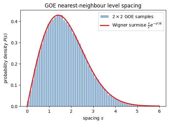
For a Hamiltonian with time-reversal symmetry the appropriate model is the Gaussian Orthogonal Ensemble, built from real symmetric matrices with random Gaussian entries. The spacing distribution is captured almost completely by the smallest nontrivial case, a \(2\times 2\) matrix. This shortcut yields the Wigner surmise \(P(s) = \tfrac{s}{2}e^{-s^2/4}\), which tracks the behavior of large matrices very closely.

The defining feature is the way the density vanishes linearly as the spacing goes to zero. Two neighboring levels rarely sit on top of each other, an effect known as level repulsion, and for this time-reversal-symmetric class the suppression grows linearly in the gap, which is characteristic of the \(\beta = 1\) symmetry index. The repulsion can be traced directly to the random-matrix weight, where coincident eigenvalues correspond to a measure-zero configuration that the distribution pushes against.

The notebook derives the surmise by integrating the GOE weight of a \(2\times 2\) matrix over its trace and angular variables, then samples random matrices to confirm the linear repulsion at small spacing.

Mathematical background

The linear repulsion has a structural origin in the change of variables from matrix entries to eigenvalues. For an invariant Gaussian ensemble the Jacobian of this transformation produces a Vandermonde factor \(\prod_{i<j}|\lambda_i - \lambda_j|^\beta\), so the joint eigenvalue density takes the log-gas form

\[ P(\lambda_1,\dots,\lambda_N) \propto \prod_{i<j}|\lambda_i-\lambda_j|^\beta\; e^{-\frac{\beta}{2}\sum_i V(\lambda_i)} , \]

a one-dimensional Coulomb gas of eigenvalues that repel logarithmically, with \(\beta^{-1}\) acting as a temperature. The exponent \(\beta\) is the Dyson index, fixed by time-reversal symmetry through the threefold way: \(\beta = 1\) for time-reversal-invariant systems with \(T^2 = +1\) (orthogonal, GOE), \(\beta = 2\) when time-reversal is broken (unitary, GUE), and \(\beta = 4\) for \(T^2 = -1\) (symplectic, GSE). The small-spacing repulsion inherits this exponent, \(P(s) \propto s^\beta\) as \(s \to 0\), so the linear growth of the GOE surmise is the \(\beta = 1\) case. On larger scales the same correlations appear as spectral rigidity, measured by the number variance \(\Sigma^2(L) = \langle (N(L) - L)^2\rangle\) of the unfolded spectrum, which grows only logarithmically for chaotic spectra against the linear \(\Sigma^2(L) = L\) of an uncorrelated Poisson spectrum.

Exercise

Consider a \(2 \times 2\) GOE matrix \(H = \begin{pmatrix} a & c \\ c & b \end{pmatrix}\) with GOE measure \(P(H) \propto \exp\bigl(-\mathrm{Tr}(H^2)/2\bigr)\).

(a) Write down the joint distribution \(P(a, b, c)\).

(b) Find the energy spacing \(s = \lambda_+ - \lambda_-\) in terms of \(a, b, c\).

(c) Change variables to \(t = a+b\), \(x = a-b\), \(y = 2c\). Integrate out the trace and the angular variable to derive \(P(s) \propto s\, e^{-s^2/4}\).

Solution

Part (a): Joint distribution

The trace of \(H^2\) is:

\[ \mathrm{Tr}(H^2) = a^2 + b^2 + 2c^2. \]

(The factor 2 on \(c^2\) arises because \(c\) appears both above and below the diagonal.) The GOE measure is:

\[ P(a, b, c) \propto \exp\!\left(-\frac{a^2 + b^2 + 2c^2}{2}\right). \]

This means \(a, b \sim \mathcal{N}(0, 1)\) independently, and \(c \sim \mathcal{N}(0, 1/2)\) (the off-diagonal has half the variance).

Part (b): Spacing formula

The eigenvalues of the \(2 \times 2\) symmetric matrix are:

\[ \lambda_\pm = \frac{a + b}{2} \pm \sqrt{\frac{(a-b)^2}{4} + c^2}. \]

The spacing is:

\[ s = \lambda_+ - \lambda_- = 2\sqrt{\frac{(a-b)^2}{4} + c^2} = \sqrt{(a-b)^2 + 4c^2}. \]

Part (c): Deriving the Wigner surmise

Step 1: Change variables. Let \(t = a + b\), \(x = a - b\), \(y = 2c\). Then \(a = (t+x)/2\), \(b = (t-x)/2\), \(c = y/2\), and:

\[ a^2 + b^2 + 2c^2 = \frac{t^2 + x^2}{2} + \frac{y^2}{2} = \frac{t^2 + x^2 + y^2}{2}. \]

The Jacobian is \(|\partial(a,b,c)/\partial(t,x,y)| = 1/4\). The distribution becomes:

\[ P(t, x, y) \propto \exp\!\left(-\frac{t^2}{4}\right) \cdot \exp\!\left(-\frac{x^2 + y^2}{4}\right). \]

Step 2: Integrate out the trace. The variable \(t\) (the trace \(\mathrm{Tr}(H)\)) decouples completely and integrates to a constant \(\int e^{-t^2/4}\,dt = 2\sqrt{\pi}\).

Step 3: Switch to polar coordinates. The spacing is \(s = \sqrt{x^2 + y^2}\). In polar coordinates \((s, \theta)\) with \(x = s\cos\theta\), \(y = s\sin\theta\):

\[ dx\,dy = s\,ds\,d\theta. \]

Integrating over the angle \(\theta \in [0, 2\pi)\) gives a factor \(2\pi\):

\[ \boxed{P(s) = \frac{s}{2}\,e^{-s^2/4}, \qquad s \geq 0.} \]

(Normalization: \(\int_0^\infty \frac{s}{2} e^{-s^2/4}\,ds = 1\), verified by substitution \(u = s^2/4\).)

Physical interpretation: The factor \(s\) in \(P(s) \propto s\) as \(s \to 0\) is the linear level repulsion of the GOE (\(\beta = 1\)). Compare: the GUE has \(P(s) \propto s^2\) (quadratic; the same \(\beta = 2\) repulsion appears for the CUE in Exercise 2.3), and the Poisson ensemble (no correlations) has \(P(s) \propto \text{const}\) (no repulsion).

---

Symbolic Verification (SymPy)

Code

import sympy as sp

s = sp.Symbol('s', positive=True)

P_wigner = s/2 * sp.exp(-s**2/4)
norm = sp.integrate(P_wigner, (s, 0, sp.oo))
print(f"∫₀^∞ P(s) ds = {norm}")
assert norm == 1

# Mean spacing
mean_s = sp.integrate(s * P_wigner, (s, 0, sp.oo))
print(f"⟨s⟩ = {mean_s} = {sp.nsimplify(mean_s)}")

# Mode (most probable spacing): dP/ds = 0
dP = sp.diff(P_wigner, s)
mode = sp.solve(dP, s)
print(f"Mode: s* = {mode} = √2 = {sp.sqrt(2)}")

∫₀^∞ P(s) ds = 1
⟨s⟩ = sqrt(pi) = sqrt(pi)
Mode: s* = [sqrt(2)] = √2 = sqrt(2)

---

Numerical Verification

Code

import numpy as np

np.random.seed(42)
n_samples = 100000

# Sample 2x2 GOE and compute spacings
spacings = []
for _ in range(n_samples):
    a, b = np.random.randn(2)
    c = np.random.randn() / np.sqrt(2)
    s = np.sqrt((a-b)**2 + 4*c**2)
    spacings.append(s)

spacings = np.array(spacings)

# Compare histogram to Wigner surmise
bins = np.linspace(0, 6, 60)
centers = (bins[:-1] + bins[1:]) / 2
hist, _ = np.histogram(spacings, bins=bins, density=True)
P_theory = centers/2 * np.exp(-centers**2/4)

residual = np.max(np.abs(hist - P_theory))
print(f"Max |histogram − P(s)| = {residual:.4f}")
assert residual < 0.02

# Verify P(0) → 0: fraction with s < 0.1
frac_small = np.mean(spacings < 0.1)
print(f"Fraction with s < 0.1: {frac_small:.4f} (linear repulsion)")

print(f"⟨s⟩ = {np.mean(spacings):.4f} (theory: √π ≈ {np.sqrt(np.pi):.4f})")
print("\nWigner surmise (GOE) confirmed.")

Max |histogram − P(s)| = 0.0091
Fraction with s < 0.1: 0.0026 (linear repulsion)
⟨s⟩ = 1.7696 (theory: √π ≈ 1.7725)

Wigner surmise (GOE) confirmed.

Code

%matplotlib inline
import matplotlib.pyplot as plt

fig, ax = plt.subplots(figsize=(6, 4))
ax.hist(spacings, bins=bins, density=True, alpha=0.6,
        color='steelblue', edgecolor='white', label='$2\\times 2$ GOE samples')
s_grid = np.linspace(0, 6, 400)
ax.plot(s_grid, s_grid/2 * np.exp(-s_grid**2/4), 'r-', lw=2,
        label=r'Wigner surmise $\frac{s}{2}e^{-s^2/4}$')
ax.set_xlabel('spacing $s$')
ax.set_ylabel('probability density $P(s)$')
ax.set_title('GOE nearest-neighbour level spacing')
ax.legend()
plt.show()

Takeaway

The \(2 \times 2\) GOE reproduces the Wigner surmise \(P(s) = \tfrac{s}{2}e^{-s^2/4}\), with linear repulsion \(P(s) \propto s\) near zero. The histogram of sampled spacings tracks this curve across the full range.

Connections

Level repulsion is the static, spectral face of quantum chaos. The same correlations that keep neighbouring levels apart in the histogram here also govern the dynamics, and their Fourier transform is the ramp of the spectral form factor. A notebook about energy gaps and a notebook about late-time dynamics are therefore looking at one object from two sides. Within random matrix theory, the semicircle law fixes the overall shape of the spectrum and the CUE eigenphase repulsion shows the same physics for unitaries rather than Hamiltonians.

References

• Dyson, The threefold way. Algebraic structure of symmetry groups and ensembles in quantum mechanics, Journal of Mathematical Physics (1962).
• Bohigas et al., Characterization of chaotic quantum spectra and universality of level fluctuation laws, Physical Review Letters (1984).
• Atas et al., Distribution of the Ratio of Consecutive Level Spacings in Random Matrix Ensembles, Physical Review Letters (2013).
• Mehta, Random matrices, Academic Press (2004).
• Płodzień, Information Scrambling, Quantum Chaos, and Haar-Random States, lecture notes (2025). arXiv:2511.14397