The spectral form factor is built from the trace \(\mathrm{Tr}\,e^{-iHt}\), the sum of phases \(e^{-iE_n t}\) running over the energy levels of a Hamiltonian \(H\). Its magnitude squared, \(K(t) = |\mathrm{Tr}\,e^{-iHt}|^2\), expands into a double sum over pairs of levels weighted by their energy differences, which is why it serves as a probe of how the levels are correlated. Quantum chaos leaves a characteristic imprint on these correlations, and the form factor is one of the simplest places to read it.
At \(t=0\) every phase aligns and the \(D^2\) terms add coherently, giving \(K(0) = D^2\) for a spectrum of \(D\) levels. As time advances the off-diagonal terms, carrying nonzero energy differences, oscillate and interfere away. Only the \(D\) diagonal terms, where a level is paired with itself, contribute a steady value, so the long-time average settles at \(\overline{K} = D\). The ratio \(K(0)/\overline{K} = D\) records how much coherence was present at the start.
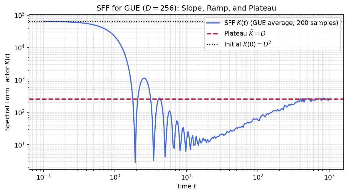
Between these two ends the averaged form factor traces a recognizable shape. It first dips below its initial value, then climbs along a linear ramp before flattening into the plateau at \(D\). The ramp is the fingerprint of level repulsion, the tendency of chaotic spectra to avoid near-degeneracies, while the plateau height counts levels and nothing more.
The notebook derives the plateau value by time-averaging the double sum and isolating the diagonal terms, then samples random Hamiltonians from the Gaussian unitary ensemble to show how the dip and ramp give way to the plateau pinned at \(K = D\).
Mathematical background
It helps to write the form factor as the squared modulus of a complex-time partition function. With \(Z(\beta + it) = \mathrm{Tr}\,e^{-(\beta+it)H} = \sum_n e^{-(\beta+it)E_n}\), the spectral form factor is
Setting \(\beta = 0\) isolates the spectral content. The double sum splits into a diagonal part (\(m=n\)), which contributes the constant \(D\), and an off-diagonal part that depends on the distribution of level differences \(E_m - E_n\). For an uncorrelated (Poisson) spectrum the off-diagonal phases average to a fast decay with no ramp. For a chaotic spectrum the two-level correlations of the unitary (\(\beta = 2\)) ensemble instead produce a linear-in-time ramp, \(K(t) \propto t\), that rises until the Heisenberg time \(t \sim D\) and then saturates at the plateau \(\overline{K} = D\). The ramp is the time-domain image of level repulsion, and the plateau height counts the number of levels, so the whole dip-ramp-plateau curve is fixed by the spectral statistics alone and is blind to the choice of operator.
Motivation
The spectral form factor (SFF) \(K(t) = |Z(it)|^2 = |\mathrm{Tr}(e^{-iHt})|^2\) is the spectral diagnostic of quantum chaos. It probes pair correlations of energy levels. The SFF exhibits three regimes: a slope (dip below \(D^2\)), a ramp (linear in \(t\), reflecting level repulsion), and a plateau at \(K = D\). This exercise derives the plateau value from time-averaging and relates it to the dephasing of off-diagonal terms.
Preliminaries / Toolbox
1. Spectral Form Factor (SFF): Provides a proxy for the analytic continuation of the partition function to study late-time chaos geometry. \(K(t) = |Z(i t)|^2 = |\mathrm{Tr}(e^{-i H t})|^2 = \sum_{m,n} e^{-i(E_m - E_n)t}\).
2. Level Repulsion: In chaotic models (like GUE), eigenvalues repel each other (\(P(\Delta E) \sim \Delta E^\beta \to 0\)). They never perfectly cross.
3. Time Averaging: Off-diagonal terms \(e^{-i(E_m - E_n)t}\) strongly oscillate and vanish under time average, isolating diagonal contributions.
4. Coherence vs Dephasing:\(K(0) = D^2\) shows full coherence, while \(K \to D\) indicates full dephasing into mutually orthogonal eigenvectors.
Exercise
For a \(D \times D\) GUE Hamiltonian with eigenvalues \(\{E_n\}\): \(K(t) = \sum_{m,n} e^{-it(E_m - E_n)}\).
(a) Show the long-time average \(\overline{K} = D\).
(b) Explain why \(K_{\mathrm{plateau}} = D\) (not \(D^2\)) and interpret the ratio \(K(0)/\overline{K}\).
GUE level repulsion ensures \(\omega_{mn} \neq 0\) with probability 1 (eigenvalues don’t coincide).
\[
\boxed{\overline{K} = D.}
\]
Part (b): Interpretation
At \(t = 0\): all \(D^2\) terms contribute coherently, \(K(0) = D^2\).
At late times: the \(D(D-1)\) off-diagonal terms dephase (oscillate with incommensurate frequencies and cancel upon averaging), leaving only the \(D\) diagonal terms.
The ratio:
\[
\frac{K(0)}{\overline{K}} = \frac{D^2}{D} = D
\]
quantifies the coherent enhancement at \(t = 0\). This dephasing from \(D^2\) to \(D\) is the spectral signature of quantum chaos, the loss of coherence between energy eigenstates over time.
Symbolic Verification (SymPy)
Code
import sympy as spD, t = sp.symbols('D t', positive=True)# SFF: K(t) = |Tr(e^{-iHt})|^2 = sum_{m,n} e^{-i(E_m - E_n)t}# Time average: <K> = sum_{m,n} delta(E_m, E_n) * 1# For non-degenerate spectrum: <K> = D (only diagonal terms survive)print('Spectral Form Factor time average:')print(f' K(0) = |Tr(I)|^2 = D^2')print(f' <K>_T = D (diagonal terms only, non-degenerate)')print(f' Ratio K(0)/<K> = D')# Numerical checkfor n inrange(2, 8): d =2**nprint(f' N={n}: K(0)={d**2}, <K>={d}, ratio={d}')
Spectral Form Factor time average:
  K(0) = |Tr(I)|^2 = D^2
  <K>_T = D  (diagonal terms only, non-degenerate)
  Ratio K(0)/<K> = D
  N=2: K(0)=16, <K>=4, ratio=4
  N=3: K(0)=64, <K>=8, ratio=8
  N=4: K(0)=256, <K>=16, ratio=16
  N=5: K(0)=1024, <K>=32, ratio=32
  N=6: K(0)=4096, <K>=64, ratio=64
  N=7: K(0)=16384, <K>=128, ratio=128
Numerical Verification
Code
import numpy as npnp.random.seed(42)for D in [4, 8, 16, 32]: A = np.random.randn(D,D) +1j*np.random.randn(D,D) H = (A + A.conj().T) / (2*np.sqrt(D)) E = np.linalg.eigvalsh(H)# SFF at 1000 time points and average times = np.linspace(10, 500, 1000) K_vals = [abs(np.sum(np.exp(-1j*E*t)))**2for t in times] K_bar = np.mean(K_vals)print(f"D={D:3d}: K(0)={D**2:5d}, K̄={K_bar:8.2f}, K̄/D={K_bar/D:.3f}")assertabs(K_bar/D -1) <0.15print("\nSFF plateau at K̄ = D confirmed.")
import matplotlib.pyplot as plt# A single GUE realization is too noisy to expose the ramp; averaging the SFF# over many independent samples reveals the dip-ramp-plateau structure, with the# linear ramp set by level repulsion and the plateau pinned at K = D.np.random.seed(45)D =256reps =200times_log = np.logspace(-1, 3, 250)K_sum = np.zeros(len(times_log))for _ inrange(reps): A = np.random.randn(D, D) +1j*np.random.randn(D, D) H = (A + A.conj().T) / (2*np.sqrt(D)) E = np.linalg.eigvalsh(H) K_sum += np.abs(np.exp(-1j*np.outer(times_log, E)).sum(axis=1))**2K = K_sum / repsplt.rcParams['figure.dpi'] =150plt.figure(figsize=(8, 4.5))plt.loglog(times_log, K, color='royalblue', linewidth=1.8, label=f'SFF $K(t)$ (GUE average, {reps} samples)')plt.axhline(D, color='crimson', linestyle='--', linewidth=2, label=r'Plateau $\bar{K} = D$')plt.axhline(D**2, color='black', linestyle=':', label=r'Initial $K(0) = D^2$')plt.xlabel(r"Time $t$")plt.ylabel(r"Spectral Form Factor $K(t)$")plt.title(f"SFF for GUE ($D={D}$): Slope, Ramp, and Plateau")plt.legend()plt.grid(True, which="both", ls="--", alpha=0.5)plt.tight_layout()plt.show()
Takeaway
The long-time average of the spectral form factor equals \(D\), the number of diagonal terms that outlive dephasing, and the ratio \(K(0)/\overline{K} = D\) measures the coherence present at \(t = 0\). The plot shows the slope and ramp giving way to a plateau pinned at \(K = D\).
Connections
The ramp of the spectral form factor is the time-domain image of the level rigidity that the GOE spacing distribution measures statically, so the same two-level correlations appear once in a histogram of gaps and once in a curve against time. The plateau, where the form factor saturates at the Hilbert space dimension, reflects the discreteness of the spectrum and is what separates a finite quantum system from a continuous one.
References
Gharibyan et al., Onset of random matrix behavior in scrambling systems, Journal of High Energy Physics (2018).
Chan et al., Solution of a Minimal Model for Many-Body Quantum Chaos, Phys. Rev. X (2018).
Cotler et al., Black holes and random matrices, Journal of High Energy Physics (2017).
Kos et al., Many-Body Quantum Chaos: Analytic Connection to Random Matrix Theory, Physical Review X (2018).
Płodzień, Information Scrambling, Quantum Chaos, and Haar-Random States, lecture notes (2025). arXiv:2511.14397