Classifying a Topological (SPT) Phase with a Quantum Extreme Learning Machine
A standalone worked example. We take the ground state of a many-body chain that hosts a symmetry-protected topological (SPT) phase, push it once through a fixed quantum “reservoir”, read out a handful of low-weight Pauli expectation values, and train only a linear classifier on top. The twist that makes this example sharper than its symmetry-breaking cousin: the SPT phase has no local order parameter, so a linear readout on the bare observables is at chance. After a fixed scramble, the same readout separates the phases and its decision boundary lands near the true critical point. Scrambling is what makes the topological order locally measurable.
Motivation: order without a local order parameter
A conventional (Landau) phase transition is signalled by a local order parameter: an observable that is nonzero in one phase and vanishes in the other, tied to a broken symmetry. A symmetry-protected topological (SPT) phase breaks no symmetry. Its two phases cannot be told apart by any local order parameter at all; the distinction lives in a nonlocal string and in the entanglement structure.
The cluster-Ising chain is the cleanest example. In the SPT (cluster) phase the ground state is a cluster state, whose order is stored in a string operator spanning the whole chain. Every conventional local order parameter, the magnetizations and the short-range correlators, is identically zero in both phases. This is exactly the obstruction the chapter is about: the phase information is present in the state but invisible to local measurements.
A Quantum Extreme Learning Machine (QELM) turns the obstruction into a tool:
The input is a quantum state, the ground state \(|\psi_{\rm gs}(h)\rangle\).
A fixed, untrained scrambling unitary spreads its information across the register.
We measure a fixed bank of simple, low-weight observables to form a feature vector.
Only a classical linear readout is trained.
Under the scramble a low-weight observable \(O\) becomes the high-weight \(U^\dagger O U\), which overlaps the nonlocal string order. So the fixed, generic scramble rotates the hidden topological order into ordinary low-weight expectation values, and a linear readout on them succeeds where the bare readout could not.
Problem statement
Model. The cluster-Ising chain on an open chain of \(N\) spins, \[
H(h) = -J\sum_{i} Z_{i-1} X_i Z_{i+1} \;-\; h \sum_i X_i .
\] It has a quantum phase transition at \(h/J = 1\):
\(h < 1\): SPT / cluster phase (the three-body cluster term dominates).
\(h > 1\): trivial paramagnet (the transverse field dominates).
Protecting symmetry.\(H(h)\) commutes with the two sublattice parities \(P_{\rm even} = \prod_{i\ {\rm even}} X_i\) and \(P_{\rm odd} = \prod_{i\ {\rm odd}} X_i\), generating a \(\mathbb{Z}_2 \times \mathbb{Z}_2\) symmetry that protects the SPT phase.
Task. Given only the ground state at a field \(h\), decide which phase it is in, training only far from criticality and never using an order parameter.
QELM protocol (per input \(h\)). 1. Diagonalize \(H(h)\) (in the symmetry sector) and take the ground state. 2. Evolve under a fixed nonintegrable scrambling unitary \(U = e^{-i H_{\rm res} t}\). 3. Read a fixed bank of low-weight Pauli expectations \(f_\alpha = \langle \psi_{\rm gs}| U^\dagger O_\alpha U |\psi_{\rm gs}\rangle\). 4. Fit a linear (logistic) readout on \(f\) to predict the phase label.
Code
import numpy as npfrom scipy.linalg import expm, eighfrom sklearn.linear_model import LogisticRegressionfrom sklearn.preprocessing import StandardScalerfrom sklearn.decomposition import PCAimport matplotlib.pyplot as pltnp.set_printoptions(precision=3, suppress=True)I2 = np.eye(2, dtype=complex)X = np.array([[0, 1], [1, 0]], dtype=complex)Y = np.array([[0, -1j], [1j, 0]], dtype=complex)Z = np.array([[1, 0], [0, -1]], dtype=complex)def kron_op(single, site, N): op = np.array([[1.0]], dtype=complex)for j inrange(N): op = np.kron(op, single if j == site else I2)return opdef kron_string(ops_by_site, N): op = np.array([[1.0]], dtype=complex)for j inrange(N): op = np.kron(op, ops_by_site.get(j, I2))return op
The model Hamiltonian, its symmetry, and a unique ground state
We build \(H(h)\) densely (for \(N=8\) the Hilbert space is only \(2^8 = 256\) dimensional). Two subtleties make the SPT chain different from the transverse-field Ising case.
Edge modes. On an open chain the cluster term only runs over the \(N-2\) interior sites, so the pure cluster Hamiltonian has a four-fold degenerate ground space (the hallmark of the SPT phase: protected edge modes). A bare diagonalizer would return an arbitrary mixture inside this near-degenerate space, washing out the string order. We remove the ambiguity by projecting onto the \((P_{\rm even}, P_{\rm odd}) = (+1,+1)\) symmetry sector (the sector that also contains the trivial all-\(|+\rangle\) state), which selects one unique, symmetric ground state.
No local order parameter. In the symmetric ground state the single-site magnetizations \(\langle Z_i\rangle, \langle Y_i\rangle\) and the nearest-neighbour correlators \(\langle Z_iZ_{i+1}\rangle, \langle Y_iY_{i+1}\rangle\) are zero in both phases, forbidden by the protecting symmetry. We verify this below.
Code
def cluster_ising(N, J, h):# H(h) = -J sum Z_{i-1} X_i Z_{i+1} - h sum X_i on an open chain H = np.zeros((2**N, 2**N), dtype=complex)for i inrange(1, N -1): H +=-J * (kron_op(Z, i -1, N) @ kron_op(X, i, N) @ kron_op(Z, i +1, N))for i inrange(N): H +=-h * kron_op(X, i, N)return Hdef sublattice_parity(N): Pe = np.eye(2**N, dtype=complex); Po = np.eye(2**N, dtype=complex)for s inrange(N):if s %2==0: Pe = Pe @ kron_op(X, s, N)else: Po = Po @ kron_op(X, s, N)return Pe, Podef symmetry_projector(N): Pe, Po = sublattice_parity(N)return ((np.eye(2**N) + Pe) /2) @ ((np.eye(2**N) + Po) /2)def ground_state(N, J, h, Proj, lam=50.0):# lift every other symmetry sector by lam; the (+1,+1) sector is untouched w, v = eigh(cluster_ising(N, J, h) + lam * (np.eye(2**N) - Proj))return v[:, 0].astype(complex)N, J =8, 1.0Proj = symmetry_projector(N)# Verify: the conventional local order parameters vanish in BOTH phases.for h in (0.2, 1.8): psi = ground_state(N, J, h, Proj) z0 = np.vdot(psi, kron_op(Z, N//2, N) @ psi).real zz = np.vdot(psi, (kron_op(Z, N//2, N) @ kron_op(Z, N//2+1, N)) @ psi).realprint(f"h={h}: <Z_i>={z0:+.2e} <Z_i Z_i+1>={zz:+.2e} (both ~0, symmetry-forbidden)")
The order that does distinguish the phases is the product of the bulk cluster stabilizers \(K_i = Z_{i-1} X_i Z_{i+1}\). Multiplying them along the chain telescopes the \(Z\)’s and leaves \[
S = \big\langle\, Z_1\, Y_2\, X_3 \cdots X_{N-2}\, Y_{N-1}\, Z_N \,\big\rangle ,
\] a weight-\(N\) string: \(Z\) on the two ends, \(Y\) just inside, \(X\) across the bulk. (The field-along-\(X\) convention puts \(Y\)’s next to the \(Z\) endpoints; a naive \(Z\!\cdots\!Z\) string is identically zero here.) \(S \approx 1\) on the ideal cluster state and decays to \(0\) in the trivial phase. Crucially \(S\) is nonlocal: it is in no low-weight bank and cannot be read from local measurements on the bare state.
Code
def string_operator(N): ops = {0: Z, N-1: Z, 1: Y, N-2: Y}for j inrange(2, N-2): ops[j] = Xreturn kron_string(ops, N)Sop = string_operator(N)for h in (0.05, 0.5, 2.0): psi = ground_state(N, J, h, Proj)print(f"h={h}: string order S = {np.vdot(psi, Sop @ psi).real:+.3f}")
h=0.05: string order S = +0.995
h=0.5: string order S = +0.487
h=2.0: string order S = +0.001
The fixed reservoir: a symmetry-breaking scrambler
For the input to be usefully re-expressed in low-weight observables the reservoir must scramble. A pure transverse-field Ising model is Jordan-Wigner integrable and does not scramble; adding a longitudinal field breaks integrability. A second requirement appears here: the reservoir must also break the protecting \(\mathbb{Z}_2\times\mathbb{Z}_2\) symmetry. If it did not, \(U^\dagger O U\) would stay in the symmetry-forbidden sector and its expectation would remain exactly zero, no matter how strongly the reservoir mixed the state.
The mixed-field Ising chain \(H_{\rm res} = J_r \sum_i Z_i Z_{i+1} + h_x \sum_i X_i + h_z \sum_i Z_i\) does both: the longitudinal \(h_z\) breaks integrability and the cluster symmetry. We fix its parameters and the evolution time once; nothing in the reservoir is trained.
Code
def mixed_field_ising(N, Jr, hx, hz): H = np.zeros((2**N, 2**N), dtype=complex)for i inrange(N -1): H += Jr * (kron_op(Z, i, N) @ kron_op(Z, i +1, N))for i inrange(N): H += hx * kron_op(X, i, N) + hz * kron_op(Z, i, N)return HJR, HX, HZ, T_EV =1.0, 1.05, 0.5, 2.5U = expm(-1j* mixed_field_ising(N, JR, HX, HZ) * T_EV) # fixed oncePe, Po = sublattice_parity(N)Hres = mixed_field_ising(N, JR, HX, HZ)print("U unitary?", np.allclose(U.conj().T @ U, np.eye(2**N)))print("reservoir breaks the cluster symmetry?", not np.allclose(Hres @ Pe, Pe @ Hres))
U unitary? True
reservoir breaks the cluster symmetry? True
The fixed measurement bank: symmetry-forbidden local observables
We read a bank of low-weight observables that are exactly the conventional local order-parameter candidates: single-site \(\{Y_i, Z_i\}\) and nearest-neighbour \(\{Y_iY_{i+1}, Z_iZ_{i+1}\}\). Every one of them is forbidden by the protecting symmetry, so on the bare ground state it vanishes in both phases. For a pure state \(\psi\), a Pauli string \(P = i^{p} X^{x} Z^{z}\) has \(\langle P\rangle = \mathrm{Re}\sum_b \overline{\psi_b}\, W_b\, \psi_{b\oplus x}\), an \(O(2^N)\) contraction we vectorize over the whole bank at once.
Code
_POP = np.array([bin(i).count('1') for i inrange(1<<16)])_PH = np.array([1, 1j, -1, -1j])def pauli_readout(N): bit =lambda i: 1<< (N -1- i) specs, names = [], []for i inrange(N): specs += [(bit(i), bit(i), 1), (0, bit(i), 0)] # Y_i, Z_i names += [f'Y{i}', f'Z{i}']for i inrange(N -1): m = bit(i) | bit(i +1) specs += [(m, m, 2), (0, m, 0)] # Y_iY_{i+1}, Z_iZ_{i+1} names += [f'Y{i}Y{i+1}', f'Z{i}Z{i+1}'] b = np.arange(1<< N) COLS = np.array([b ^ x for (x, z, p) in specs]) W = np.array([_PH[p] * (1-2* (_POP[z & b] &1)) for (x, z, p) in specs], dtype=complex)return COLS, W, namesCOLS, W, names = pauli_readout(N)print(f"{len(names)} symmetry-forbidden features, e.g. {names[:2]} ... {names[-2:]}")
30 symmetry-forbidden features, e.g. ['Y0', 'Z0'] ... ['Y6Y7', 'Z6Z7']
The feature map, and why the bare readout is blind
For each input \(h\) we form the symmetric ground state and read the bank either on the bare state or on the scrambled state \(\phi = U\psi\). The bare features vanish to machine precision; the scrambled features are \(O(0.1)\) and carry the string order.
Code
def qelm_features(psi_list, U, COLS, W): F = np.zeros((len(psi_list), COLS.shape[0]))for n, psi inenumerate(psi_list): phi = U @ psi if U isnotNoneelse psi F[n] = np.real(np.conj(phi) * W * phi[COLS]).sum(axis=1)return Fpsi_demo = ground_state(N, J, 0.2, Proj)f_bare = qelm_features([psi_demo], None, COLS, W)f_scram = qelm_features([psi_demo], U, COLS, W)print("deep-SPT input h=0.2:")print(f" |bare features| max = {np.abs(f_bare).max():.1e} (zero: symmetry-forbidden)")print(f" |scrambled feat.| max = {np.abs(f_scram).max():.3f} (nonzero: carries the string order)")
deep-SPT input h=0.2:
  |bare features|   max = 5.0e-16   (zero: symmetry-forbidden)
  |scrambled feat.| max = 0.152   (nonzero: carries the string order)
Train far from criticality, test across the transition
We draw training fields only from the clearly-SPT (\(h \in [0.05, 0.55]\)) and clearly-trivial (\(h \in [1.45, 2.5]\)) windows, label them \(0/1\), hold out a separate set of clear-region fields for honest accuracy, and use a dense sweep to probe the critical region the readout never trained on.
Train the linear readout on the scrambled features
The only trainable object is a logistic-regression readout on the standardized scrambled features. Because each feature \(f_\alpha = \mathrm{Tr}(\rho\,U^\dagger O_\alpha U)\) is linear in the state\(\rho\), a linear readout is the well-posed choice.
The ablation: bare vs scrambled, under finite shots
A real device estimates each expectation from a finite number of measurement shots, with variance \((1-\langle O\rangle^2)/M\). On the bare forbidden features (true value zero) this is pure noise, so the readout is at chance no matter how many shots are taken. On the scrambled features the \(O(0.1)\) signal survives easily. We average the accuracy over shot-noise realizations for a fair, identical comparison.
Visualize: manifold, decision boundary, and the physics behind the ablation
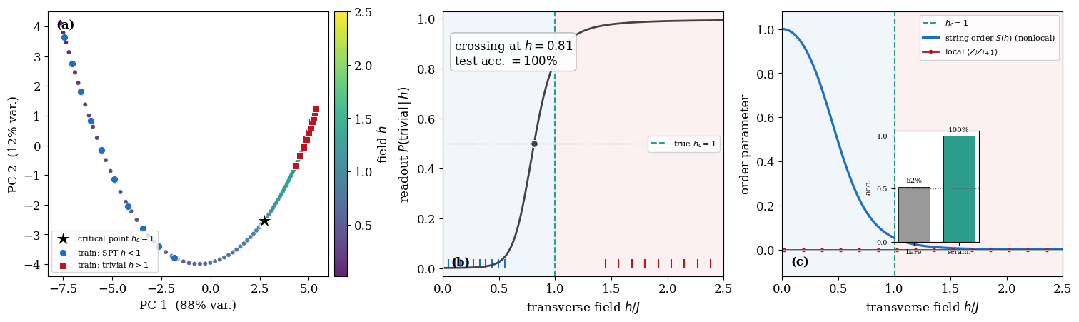
Panel (a): a 2D PCA of the scrambled feature vectors, a smooth arc parametrized by \(h\), with the SPT and trivial training states apart. Panel (b): the readout’s predicted trivial probability, crossing near \(h_c\). Panel (c): the nonlocal string order \(S(h)\) dropping across \(h_c\) while the local order parameter stays at zero, plus the bare-vs-scrambled accuracies.
What happened. A fixed, untrained scramble turned each ground state into a feature vector of ordinary low-weight expectation values. A linear readout, trained only on states far from the transition, learned the boundary between the SPT and trivial phases and placed it near the true critical point \(h_c = 1\), without ever being handed an order parameter.
Why the bare readout fails. The SPT phase breaks no symmetry, so every low-weight observable in our bank is forbidden by the protecting \(\mathbb{Z}_2\times\mathbb{Z}_2\) symmetry and vanishes identically in both phases. The phase information lives only in the nonlocal weight-\(N\) string order \(S\). A linear readout on the bare features has no signal, and under finite shots it sits at chance.
Why scrambling fixes it. Under \(U\) a low-weight \(O\) becomes the high-weight \(U^\dagger O U\). Because the reservoir does not share the protecting symmetry, this scrambled observable is no longer forced to vanish, and it overlaps the string order. The same low-weight readout, now on the scrambled features, inherits the topological order and separates the phases. This is the chapter’s thesis made concrete: scrambling turns the obstruction (nonlocality) into the tool (local measurability).
A sharper statement. It is specifically the reservoir’s symmetry breaking, not scrambling alone, that unlocks the order. A symmetry-respecting scrambler, however strong, keeps \(U^\dagger O U\) in the forbidden sector, so the scrambled features stay exactly zero and the readout stays at chance. The reader can verify this by replacing \(H_{\rm res}\) with a cluster-plus-transverse Hamiltonian that commutes with \(P_{\rm even}, P_{\rm odd}\).
Connection to typicality and scrambling. This is the same mechanism that runs through the book. A generic, structureless (Haar-like) time evolution spreads localized information across the whole register; here that spreading is exactly what maps a nonlocal invariant into locally accessible observables. The QELM does not compute the string order; it lets the reservoir’s scrambling dynamics express it in the bank of observables a real device can measure.
The caveat. Every feature is linear in \(\rho\), so a linear readout is well posed for any observable that is itself linear in the state. A genuinely nonlinear functional such as the entanglement entropy could not be recovered this way from single-copy expectation values, regardless of training; that requires multi-copy protocols. Phase classification here happens to be a linear-in-\(\rho\) task once the scramble has done its work.
Finite size. On an open chain of \(N=8\) the string order has already decayed substantially before \(h_c\), so the decision crossing sits somewhat below the thermodynamic \(h_c=1\). It sharpens toward \(h_c=1\) as \(N\) grows.