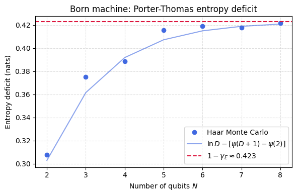
A Born machine is a generative model that produces samples the way a quantum measurement does. A circuit \(U(\boldsymbol{\theta})\) acts on \(N\) qubits, and reading out the result in the computational basis returns a bitstring \(x\) with probability \(p(x) = |\langle x|U(\boldsymbol{\theta})|0\rangle|^2\). The \(2^N\) possible outcomes carry a probability distribution, and training the model means reshaping that distribution by adjusting the angles until the samples resemble the data. How rich the distribution can get is governed by how much entanglement the circuit builds, and both ends of the entanglement range impose a limit.
With no entanglement the state is a product across qubits and the distribution factorizes, each bit decided on its own. The inverse participation ratio \(\sum_x p(x)^2\), which counts how few outcomes carry most of the weight, is then fixed entirely by the single-qubit magnetizations to \(2^{-N}\prod_j(1+m_j^2)\). It runs from \(1/D\) when the weight is spread flat to \(1\) when it all collapses onto one bitstring. A product circuit can be broad or sharp, yet it can place no correlation between qubits.
At the opposite end a circuit deep enough to form a 2-design draws from a Porter-Thomas distribution, where the individual probabilities scatter according to the law \(De^{-Dp}\), the speckle pattern of a random quantum state. Such a state is never smooth. Its Shannon entropy lands a fixed amount \(1-\gamma_E \approx 0.423\) nats below the uniform value \(\ln D\), a constant deficit set by the random-speckle statistics rather than by anything tunable.
The same entanglement that lets the model spread weight across the outcome space also caps the correlations it can carry. The classical mutual information between two registers is bounded by \(2S(\rho_A)\), twice the entanglement entropy of the cut, through the data processing inequality. Reproducing correlations between distant parts of a dataset therefore demands genuine long-range entanglement in the circuit, which ties the statistical reach of the model to a physical resource.
Motivation
A Born machine is a quantum generative model where samples are drawn from the Born probability distribution \(p(x) = |\langle x | U(\boldsymbol{\theta}) | 0\rangle|^2\). Generative modeling aims to learn complex, highly correlated probability distributions.
This exercise explores the expressivity limits of Born machines. First, product states (no entanglement) can only generate factorized distributions with limited inverse participation ratios (IPR). Second, deep chaotic circuits (unitaries forming a 2-design) generate Porter-Thomas distributions, which exhibit an “entropy deficit” relative to the uniform distribution. Finally, we prove that classical correlations in the generated distribution are strictly bounded by the quantum entanglement entropy of the underlying state.
Preliminaries / Toolbox
1. Inverse Participation Ratio (IPR):\(C_2 = \sum_x p(x)^2\). It measures the sparsity/concentration of a distribution. \(C_2 = 1\) for a delta function (completely deterministic), and \(C_2 = 1/D\) for the uniform distribution (maximally spread).
2. Porter-Thomas Distribution: For a Haar-random pure state, each Born probability \(p(x)\) is drawn from a Beta distribution \(p_x \sim \mathrm{Beta}(1, D-1)\), which approximates an exponential distribution \(\Pr(p) \approx D e^{-Dp}\) for large \(D\).
3. Beta Integral Identity: If \(x \sim \mathrm{Beta}(\alpha, \beta)\), then \(\mathbb{E}[x \ln x] = \frac{\alpha}{\alpha+\beta}\left[\psi(\alpha+1) - \psi(\alpha+\beta+1)\right]\), where \(\psi(z)\) is the digamma function.
4. Data Processing Inequality: The mutual information between classical bitstrings \(X_A\) and \(X_B\) obtained by local measurements on subsystems \(A\) and \(B\) cannot exceed the quantum mutual information \(I_Q(A:B)\) of the pre-measurement state.
Exercise
(a) Show that for a product state \(|\psi\rangle = \bigotimes_{j=1}^N |\psi_j\rangle\) with local \(Z\)-magnetizations \(m_j = \langle Z_j\rangle\), the IPR is \(C_2 = 2^{-N} \prod_j (1 + m_j^2)\). Evaluate this for (i) all \(m_j = 0\) and (ii) all \(m_j = \pm 1\).
(b) For Haar-random states, show that the average Shannon entropy is \(\mathbb{E}[H] = \psi(D+1) - \psi(2)\), and compute the entropy deficit \(\Delta_H = \ln D - \mathbb{E}[H]\).
(c) Let \(X_A\) and \(X_B\) be classical bitstrings from measuring disjoint bipartite systems \(A\) and \(B\). Prove \(I(X_A : X_B) \leq 2 S(\rho_A)\).
Solution
Part (a): IPR of a Product State
For a product state, the Born probability factorizes: \(p(x) = \prod_{j=1}^N p_j(x_j)\), where \(p_j(0) = |\alpha_j|^2\) and \(p_j(1) = |\beta_j|^2\). The magnetization is \(m_j = p_j(0) - p_j(1)\).
Since \(p_j(0) + p_j(1) = 1\), we have \(p_j(0) = \frac{1+m_j}{2}\) and \(p_j(1) = \frac{1-m_j}{2}\).
Using the asymptotic expansion of the digamma function \(\psi(z) \approx \ln z - \frac{1}{2z}\) for large \(z\), and \(\psi(2) = 1 - \gamma_E\) (where \(\gamma_E \approx 0.577\) is the Euler-Mascheroni constant):
This \(O(1)\) gap shows that Haar-random Born machines do not generate the uniform distribution; they have “speckle” fluctuations that reduce entropy.
Part (c): Entanglement bounds classical correlations
The process of drawing classical samples is conceptually a local quantum measurement map \(\mathcal{M} = \mathcal{M}_A \otimes \mathcal{M}_B\) on the pure state \(|\psi\rangle\langle\psi|\). The post-measurement classically-correlated state is \(\sigma_{AB} = \sum_{x_A, x_B} P(x_A, x_B) |x_A, x_B\rangle\langle x_A, x_B|\).
The classical mutual information is \(I(X_A : X_B) = I_Q(\sigma_{AB})\).
Because local measurements are CPTP maps, the Data Processing Inequality implies:
Consequence: A Born machine cannot learn probability distributions with long-range variable correlations (high classical mutual information) unless the underlying quantum circuit generates sufficient long-range quantum entanglement.
Symbolic Verification (SymPy)
Code
import sympy as spfrom sympy import digamma, EulerGammaD = sp.Symbol('D', positive=True, integer=True)# Part (a): IPR of product statem = sp.Symbol('m') # magnetizationC2_single = (sp.Rational(1,2) + m/2)**2+ (sp.Rational(1,2) - m/2)**2C2_simplified = sp.simplify(C2_single)print(f'Single-qubit IPR: {C2_simplified}')print(f' = (1 + m^2)/2')assert sp.simplify(C2_simplified - (1+ m**2)/2) ==0# Part (b): Porter-Thomas entropy deficit# E[H] = psi(D+1) - psi(2), deficit = 1 - gamma_Eprint(f'\nEntropy deficit = 1 - gamma_E = {float(1- EulerGamma):.4f}')# Part (c): Data processing inequalityprint(f'I(X_A:X_B) <= I_Q(A:B) = 2*S(rho_A) for pure states')
Single-qubit IPR: m**2/2 + 1/2
  = (1 + m^2)/2

Entropy deficit = 1 - gamma_E = 0.4228
I(X_A:X_B) <= I_Q(A:B) = 2*S(rho_A) for pure states
Numerical Verification
Code
%matplotlib inlineimport numpy as npimport matplotlib.pyplot as pltfrom scipy.special import digammanp.random.seed(0)gamma_E =0.5772156649N_vals = np.arange(2, 9)deficit_mc = []for N in N_vals: D =2**N Hs = []for _ inrange(400): psi = np.random.randn(D) +1j* np.random.randn(D) psi /= np.linalg.norm(psi) # Haar-random pure state p = np.abs(psi)**2 p = p[p >1e-15] Hs.append(-np.sum(p * np.log(p))) deficit_mc.append(np.log(D) - np.mean(Hs))D_exact =2.0**N_valsdeficit_exact = np.log(D_exact) - (digamma(D_exact +1) - digamma(2))plt.figure(figsize=(6, 4))plt.plot(N_vals, deficit_mc, 'o', color='royalblue', label='Haar Monte Carlo')plt.plot(N_vals, deficit_exact, '-', color='royalblue', alpha=0.6, label=r'$\ln D - [\psi(D+1)-\psi(2)]$')plt.axhline(1- gamma_E, color='crimson', ls='--', label=r'$1-\gamma_E \approx 0.423$')plt.xlabel('Number of qubits $N$')plt.ylabel('Entropy deficit (nats)')plt.title('Born machine: Porter-Thomas entropy deficit')plt.legend()plt.grid(True, ls='--', alpha=0.4)plt.tight_layout()plt.show()
Takeaway
A product state has IPR between \(1/D\) and \(1\) set by its local magnetizations, while a Haar-random Born machine follows the Porter-Thomas law and undershoots the uniform entropy by \(1-\gamma_E\approx0.423\) nats. Classical correlations between two subsystems are capped by \(2S(\rho_A)\), so a Born machine cannot reproduce long-range correlations without long-range entanglement.
Code
import numpy as npfrom scipy.special import digammafrom scipy.stats import unitary_groupnp.random.seed(42)gamma_E =0.5772156649# Part (b) Porter-Thomas Entropy Deficitprint("Part (b): Porter-Thomas Entropy Deficit of Haar-random states")print("="*65)print(f"{'N':>3s}{'D':>4s}{'E[H] MC':>10s}{'E[H] Exact':>10s}{'Deficit MC':>10s}{'1 - γ_E':>10s}")print(f"{'─'*3:>3s}{'─'*4:>4s}{'─'*10:>10s}{'─'*10:>10s}{'─'*10:>10s}{'─'*10:>10s}")for N in [3, 4, 5, 6]: D =2**N E_H_mc =0.0for _ inrange(1000): psi = unitary_group.rvs(D)[:, 0] p =abs(psi)**2 p = p[p >1e-15] E_H_mc +=-np.sum(p * np.log(p)) E_H_mc /=1000 E_H_exact = digamma(D+1) - digamma(2) H_unif = np.log(D) deficit = H_unif - E_H_mcprint(f"{N:3d}{D:4d}{E_H_mc:10.4f}{E_H_exact:10.4f}{deficit:10.4f}{1-gamma_E:10.4f}")assertabs(E_H_mc - E_H_exact) <0.05# Part (c) Mutual Information Boundprint("\nPart (c): Data Processing Bound I(X_A : X_B) <= 2S(A)")print("="*55)N =4; D =2**N; m =2**(N//2)for trial inrange(3): psi = unitary_group.rvs(D)[:, 0]# Quantum Entropy S(A) psi_mat = psi.reshape(m, m) rho_A = psi_mat @ psi_mat.conj().T eigs = np.linalg.eigvalsh(rho_A) eigs = eigs[eigs >1e-15] S_A =-np.sum(eigs * np.log(eigs))# Classical MI I(X_A : X_B) p_AB =abs(psi_mat)**2 p_A = p_AB.sum(axis=1) p_B = p_AB.sum(axis=0) I_class =0for a inrange(m):for b inrange(m):if p_AB[a,b] >1e-15: I_class += p_AB[a,b] * np.log(p_AB[a,b] / (p_A[a] * p_B[b]))print(f"Trial {trial+1}: I(X_A:X_B) = {I_class:.4f} <= 2S(A) = {2*S_A:.4f}")assert I_class <=2*S_A +1e-10
Part (b): Porter-Thomas Entropy Deficit of Haar-random states
=================================================================
  N     D     E[H] MC  E[H] Exact  Deficit MC     1 - γ_E
───  ────  ──────────  ──────────  ──────────  ──────────
  3     8      1.7081      1.7179      0.3713      0.4228
  4    16      2.3846      2.3807      0.3879      0.4228