The Shadow Channel and Its Inverse

Applications of Scrambling, numerical solution.

The Shadow Channel and Its Inverse

Background

Classical shadows learn many properties of an unknown state \(\rho\) from a handful of randomized measurements. A single shot draws a unitary \(U\) from a chosen ensemble, rotates the state by \(U\), and measures in the computational basis, recording the outcome \(b\) together with the unitary that produced it. From this record we reconstruct the snapshot \(U^\dagger |b\rangle\langle b| U\), the post-measurement state written back in the original frame. Each snapshot is a rank-one operator, cheap to store and to manipulate.

A single snapshot is random in two ways, through the draw of \(U\) and through the Born-rule outcome \(b\). Averaging the snapshot construction over the ensemble of unitaries and over the outcomes defines a linear map on operators, \[ \mathcal{M}(\rho) = \mathbb{E}_U \sum_b \langle b| U \rho U^\dagger |b\rangle\, U^\dagger |b\rangle\langle b| U, \] the measurement channel. It records what the randomized measurement reports on average when the input is \(\rho\).

When the ensemble is a unitary 2-design, such as the global Clifford group, the average can depend on \(\rho\) only through \(\rho\) itself and through \(\mathrm{Tr}(\rho)\,I\). The channel then takes the depolarizing form \[ \mathcal{M}(\rho) = \frac{\rho + \mathrm{Tr}(\rho)\,I}{D+1}, \] which leaves the trace fixed and shrinks the traceless part by the factor \(1/(D+1)\). Because no part of the operator is sent to zero, the map is invertible. 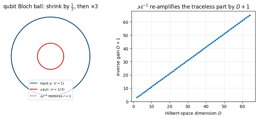Its inverse is \[ \mathcal{M}^{-1}(\tau) = (D+1)\,\tau - \mathrm{Tr}(\tau)\,I, \] and for a single qubit, \(D=2\), this reads \(\mathcal{M}^{-1}(\tau) = 3\tau - \mathrm{Tr}(\tau)\,I\). Applying \(\mathcal{M}^{-1}\) to each snapshot re-amplifies the traceless part by exactly the factor the measurement suppressed, so the corrected snapshot is an unbiased estimator of \(\rho\).

The factor \(D+1\) is the dimension of the symmetric subspace of two copies that appears in the \(k=2\) Weingarten formula, and the shrinkage it encodes is the cost of randomizing the measurement. When \(D\) is large the channel is close to singular on the traceless sector, and inverting an almost-singular channel inflates the variance of the estimator. That inflation is the price of tomographic completeness, the ability to read off any observable from the same set of snapshots.

Motivation

The shadow channel \(\mathcal{M}(\sigma) = \frac{\sigma + \mathrm{Tr}(\sigma)I}{D+1}\) arises from averaging the measure-and-prepare map over a unitary 2-design. Its invertibility is the mathematical engine of classical shadows: by applying \(\mathcal{M}^{-1}\) to each measurement outcome, we obtain an unbiased estimator of \(\rho\). This exercise derives \(\mathcal{M}\) using Weingarten calculus and verifies the inversion algebraically.

Preliminaries / Toolbox

1. Measurement Channel: Averaging over a 2-design, the preparation-measurement channel map is \(\mathcal{M}(\rho) = \mathbb{E}_{U} \sum_b \mathrm{Tr}(U \rho U^\dagger |b\rangle\langle b|) U^\dagger |b\rangle\langle b| U\).

2. Weingarten Integral (\(k=2\)): A 2-design average over polynomial degree two. Over \(D\)-dimensional space, this yields \(\mathcal{M}(\rho) = \frac{\rho + \mathrm{Tr}(\rho)I}{D+1}\).

3. Trace Properties: \(\mathrm{Tr}(A+B) = \mathrm{Tr}(A)+\mathrm{Tr}(B)\), \(\mathrm{Tr}(cI) = cD\).

4. Single Qubits: For \(D=2\), \(\mathcal{M}(\rho) = \frac{\rho + \mathrm{Tr}(\rho)I}{3}\).

Exercise

(a) For a single qubit measured in a random Clifford basis, show \(\mathcal{M}(\sigma) = \frac{\sigma + \mathrm{Tr}(\sigma)I}{3}\).

(b) Verify that \(\mathcal{M}^{-1}(\tau) = 3\tau - \mathrm{Tr}(\tau)I\) is the inverse.

(c) State the general \(D\)-dimensional formula \(\mathcal{M}(\sigma) = \frac{\sigma + \mathrm{Tr}(\sigma)I}{D+1}\) and its inverse.

Solution

Part (a): Deriving \(\mathcal{M}\) from the 2-design average

Start from the measurement channel, \[ \mathcal{M}(\rho) = \mathbb{E}_U \sum_b \langle b| U \rho U^\dagger |b\rangle\, U^\dagger |b\rangle\langle b| U . \] Each term carries two factors of \(U\) and two of \(U^\dagger\), so the average is a degree-two polynomial in the entries of \(U\). For a unitary 2-design this average equals the Haar average of the same polynomial.

The form of the channel. For any fixed \(V\) in the group, the substitution \(U \to UV^\dagger\) leaves a 2-design average unchanged, and it sends \(\rho \to V \rho V^\dagger\) while keeping the outer \(U^\dagger |b\rangle\langle b| U\) unchanged after relabeling. Hence \(\mathcal{M}(V\rho V^\dagger) = V \mathcal{M}(\rho) V^\dagger\) for every \(V\). A linear map on operators that commutes with conjugation by every unitary can only be a combination of the two invariant superoperators, the identity map and the trace map. Therefore \[ \mathcal{M}(\rho) = a\,\rho + b\,\mathrm{Tr}(\rho)\,I \] for scalars \(a\) and \(b\) that depend on \(D\) alone.

First equation, from \(\rho = I\). Setting \(\rho = I\) gives \(\sum_b U^\dagger |b\rangle\langle b| U = U^\dagger I U = I\) inside the average, so \(\mathcal{M}(I) = I\). Matching with \(a\,I + b\,\mathrm{Tr}(I)\,I = (a + bD)\,I\) yields \[ a + bD = 1 . \]

Second equation, from the second moment. Write the channel in indices, using \((U^\dagger |b\rangle\langle b| U)_{ij} = \overline{U_{bi}}\,U_{bj}\) and \(\langle b|U\rho U^\dagger|b\rangle = \sum_{kl} U_{bk}\,\rho_{kl}\,\overline{U_{bl}}\), \[ \mathcal{M}(\rho)_{ij} = \sum_{b,k,l} \rho_{kl}\; \mathbb{E}_U\!\left[\, U_{bj}\,U_{bk}\,\overline{U_{bi}}\,\overline{U_{bl}} \,\right]. \] The Haar second moment is \[ \mathbb{E}_U\!\left[\, U_{bj}\,U_{bk}\,\overline{U_{bi}}\,\overline{U_{bl}} \,\right] = \big(\mathrm{Wg}(e) + \mathrm{Wg}(\text{swap})\big)\,\big(\delta_{ij}\delta_{kl} + \delta_{il}\delta_{kj}\big), \] because all four row indices equal \(b\), so both permutations of the rows contribute equally and the column deltas supply the two pairings \(\delta_{ij}\delta_{kl}\) and \(\delta_{il}\delta_{kj}\). With the \(k=2\) Weingarten values \(\mathrm{Wg}(e) = \frac{1}{D^2-1}\) and \(\mathrm{Wg}(\text{swap}) = \frac{-1}{D(D^2-1)}\), \[ c \equiv \mathrm{Wg}(e) + \mathrm{Wg}(\text{swap}) = \frac{1}{D^2-1}\Big(1 - \frac{1}{D}\Big) = \frac{1}{D(D+1)} . \] Summing over \(b\) multiplies by \(D\), and the two pairings give \(\mathrm{Tr}(\rho)\,I\) and \(\rho\) respectively, \[ \mathcal{M}(\rho) = D\,c\,\big(\rho + \mathrm{Tr}(\rho)\,I\big) = \frac{\rho + \mathrm{Tr}(\rho)\,I}{D+1} . \] So \(a = b = \frac{1}{D+1}\), which also satisfies \(a + bD = 1\) as required.

Single qubit. For \(D = 2\), \[ \mathcal{M}(\sigma) = \frac{\sigma + \mathrm{Tr}(\sigma)\,I}{3}. \]

Part (b): Inverting the channel

Write the output as \(\tau = \mathcal{M}(\rho) = a\,\rho + b\,\mathrm{Tr}(\rho)\,I\) with \(a = b = \frac{1}{D+1}\), and solve for \(\rho\).

Recover the trace. Taking the trace of both sides and using \(\mathrm{Tr}(I) = D\), \[ \mathrm{Tr}(\tau) = (a + bD)\,\mathrm{Tr}(\rho) = \mathrm{Tr}(\rho), \] since \(a + bD = 1\). The channel preserves the trace, so \(\mathrm{Tr}(\rho)\) is read off directly from \(\tau\).

Solve for \(\rho\). Substitute \(\mathrm{Tr}(\rho) = \mathrm{Tr}(\tau)\) into \(\tau = a\,\rho + b\,\mathrm{Tr}(\rho)\,I\) and isolate \(\rho\), \[ \rho = \frac{1}{a}\big(\tau - b\,\mathrm{Tr}(\tau)\,I\big). \] With \(a = b = \frac{1}{D+1}\) this is \[ \mathcal{M}^{-1}(\tau) = (D+1)\,\tau - \mathrm{Tr}(\tau)\,I . \]

Verification. Apply \(\mathcal{M}^{-1}\) to \(\mathcal{M}(\rho)\), \[ \mathcal{M}^{-1}\!\big(\mathcal{M}(\rho)\big) = (D+1)\,\frac{\rho + \mathrm{Tr}(\rho)\,I}{D+1} - \mathrm{Tr}\!\left(\frac{\rho + \mathrm{Tr}(\rho)\,I}{D+1}\right) I . \] The first term is \(\rho + \mathrm{Tr}(\rho)\,I\). In the second term, \(\mathrm{Tr}(\rho + \mathrm{Tr}(\rho)\,I) = \mathrm{Tr}(\rho) + D\,\mathrm{Tr}(\rho) = (D+1)\,\mathrm{Tr}(\rho)\), so the second term is \(\mathrm{Tr}(\rho)\,I\). They cancel, \[ \mathcal{M}^{-1}\!\big(\mathcal{M}(\rho)\big) = \rho + \mathrm{Tr}(\rho)\,I - \mathrm{Tr}(\rho)\,I = \rho . \]

Single qubit. For \(D = 2\), \(\mathcal{M}^{-1}(\tau) = 3\,\tau - \mathrm{Tr}(\tau)\,I\). The numerical cell below applies this inverse to random matrices and confirms \(\mathcal{M}^{-1}(\mathcal{M}(\sigma)) = \sigma\) for \(D = 2, 3, 4\).

Part (c): General \(D\)-dimensional formula

\[ \boxed{\mathcal{M}(\sigma) = \frac{\sigma + \mathrm{Tr}(\sigma)\,I}{D+1}, \qquad \mathcal{M}^{-1}(\tau) = (D+1)\,\tau - \mathrm{Tr}(\tau)\,I.} \]

The channel acts as \(1/(D+1)\) on the traceless sector and fixes \(I\), which makes it trace preserving. The factor \(D+1\) is the dimension of the symmetric subspace \(\mathrm{Sym}^2(\mathbb{C}^D)\) that appears in the \(k=2\) Weingarten formula. The inverse multiplies the traceless sector back by \(D+1\), so for large \(D\) the channel is nearly singular there and the inversion amplifies fluctuations, which is the origin of the estimator variance.

Symbolic Verification (SymPy)

Code

import sympy as sp

D = sp.Symbol('D', positive=True, integer=True)

# Shadow channel from Weingarten k=2:
# M(rho) = (rho + Tr(rho)*I) / (D+1)
# Weingarten functions for S_2:
Wg_id = 1 / (D**2 - 1)
Wg_swap = -1 / (D * (D**2 - 1))
print(f'Weingarten functions for S_2:')
print(f'  Wg(id, D) = {Wg_id}')
print(f'  Wg((12), D) = {Wg_swap}')

# The k=2 twirl coefficient is D*(Wg_id + Wg_swap):
coeff = sp.simplify(D * (Wg_id + Wg_swap))
print(f'\nChannel coefficient  D*(Wg_id + Wg_swap) = {coeff}')   # = 1/(D+1)
print(f'  so  M(rho) = (rho + Tr(rho) I)/(D+1)')

# Inversion
print(f'\nInversion map: M^(-1)(tau) = (D+1)*tau - Tr(tau)*I')
print(f'  For D=2: M^(-1)(tau) = 3*tau - I')

Weingarten functions for S_2:
  Wg(id, D) = 1/(D**2 - 1)
  Wg((12), D) = -1/(D*(D**2 - 1))

Channel coefficient  D*(Wg_id + Wg_swap) = 1/(D + 1)
  so  M(rho) = (rho + Tr(rho) I)/(D+1)

Inversion map: M^(-1)(tau) = (D+1)*tau - Tr(tau)*I
  For D=2: M^(-1)(tau) = 3*tau - I

Numerical Verification

Takeaway

The shadow channel scales the traceless part of a state by \(1/(D+1)\) and leaves the identity fixed, so it inverts to \(\mathcal{M}^{-1}(\tau)=(D+1)\tau-\mathrm{Tr}(\tau)\,I\) and turns each snapshot into an unbiased estimator of \(\rho\). The factor \(D+1\) is the dimension of the symmetric subspace appearing in the \(k=2\) Weingarten formula.

Code

import numpy as np

np.random.seed(42)

for D in [2, 3, 4]:
    I_D = np.eye(D, dtype=complex)

    def M(sigma): return (sigma + np.trace(sigma)*I_D)/(D+1)
    def M_inv(tau): return (D+1)*tau - np.trace(tau)*I_D

    for trial in range(5):
        sigma = np.random.randn(D,D) + 1j*np.random.randn(D,D)
        err = np.linalg.norm(M_inv(M(sigma)) - sigma)
        assert err < 1e-12

    print(f"D={D}: M⁻¹(M(σ)) = σ verified for 5 random matrices.")

print("\nShadow channel inversion confirmed for all D.")

D=2: M⁻¹(M(σ)) = σ verified for 5 random matrices.
D=3: M⁻¹(M(σ)) = σ verified for 5 random matrices.
D=4: M⁻¹(M(σ)) = σ verified for 5 random matrices.

Shadow channel inversion confirmed for all D.

Code

# --- Visualization: the shadow channel shrinks the state, its inverse re-amplifies ---
import numpy as np
import matplotlib.pyplot as plt

fig, ax = plt.subplots(1, 2, figsize=(9, 4))

# (a) single qubit (D=2): the traceless part is scaled by 1/(D+1)=1/3, then M^-1 undoes it
theta = np.linspace(0, 2 * np.pi, 200)
ax[0].plot(np.cos(theta), np.sin(theta), color="C0", lw=2, label=r"input $\rho$  ($r=1$)")
ax[0].plot(np.cos(theta) / 3, np.sin(theta) / 3, color="C3", lw=2,
           label=r"$\mathcal{M}(\rho)$  ($r=1/3$)")
ax[0].plot(np.cos(theta), np.sin(theta), color="k", lw=1, ls="--",
           label=r"$\mathcal{M}^{-1}$ restores $r=1$")
ax[0].set_aspect("equal"); ax[0].set_xlim(-1.15, 1.15); ax[0].set_ylim(-1.15, 1.15)
ax[0].axis("off")
ax[0].set_title(r"qubit Bloch ball: shrink by $\frac{1}{3}$, then $\times 3$")
ax[0].legend(fontsize=8, loc="lower center")

# (b) the inverse gain D+1 is the variance-inflation factor, growing with D
D = np.arange(2, 65)
ax[1].plot(D, D + 1, "o-", color="C0", ms=3)
ax[1].set_xlabel(r"Hilbert-space dimension $D$")
ax[1].set_ylabel(r"inverse gain $D+1$")
ax[1].set_title(r"$\mathcal{M}^{-1}$ re-amplifies the traceless part by $D+1$")
ax[1].grid(alpha=0.3)

plt.tight_layout()
plt.show()

Connections

The averaged measurement channel built here is a Haar second moment, the same twirl that produces the Page purity and the randomized benchmarking decay. Seeing it in this form explains why the channel is invertible and why inverting it inflates the variance. The sample cost that follows from that inverse is worked out in numerical shadows.

References

Huang et al., Predicting Many Properties of a Quantum System from Very Few Measurements, Nature Physics (2020).
Elben et al., Statistical Correlations between Locally Randomized Measurements: A Toolbox for Probing Entanglement in Many-Body Quantum States, Physical Review A (2019).
Płodzień, Information Scrambling, Quantum Chaos, and Haar-Random States, lecture notes (2025). arXiv:2511.14397