Operator Averages Using the First Moment Formula

Haar Measure & Weingarten Calculus, numerical solution.

Operator Averages Using the First Moment Formula

---

Background

Conjugating an operator by a unitary, the map \(A \mapsto U A U^\dagger\), rotates it inside the space of matrices without changing its eigenvalues. The first moment asks what is left of this operator after we average the rotation over every unitary with equal weight, which is what the Haar measure prescribes. Because the average treats all directions alike, it cannot retain any information that singles out a basis, and the only quantity that survives an arbitrary rotation is the trace.

This forces the answer to be a multiple of the identity, and matching traces on both sides fixes the multiple. The result is \(\mathbb{E}_U[U A U^\dagger] = \frac{\mathrm{Tr}(A)}{D}\,I\), where \(D\) is the dimension. Read as a physical process this is complete depolarization, where the averaged rotation drives any input toward the maximally mixed state while keeping its normalization. Read through representation theory it is Schur’s lemma, since an operator commuting with every unitary must be proportional to the identity.

In the language of the Weingarten calculus this is the \(k=1\) case, the simplest instance of a general rule that turns Haar averages into sums over permutations. Here there is only one permutation to sum, so the combinatorics stays invisible, yet the same logic organizes every higher moment that follows. The identity also names the operation called twirling, which recurs whenever one averages a fixed observable against a randomly chosen frame.

The notebook puts the formula to work on \(\mathbb{E}_U[\mathrm{Tr}(U A U^\dagger B)]\), a contraction of the rotated operator against a second fixed matrix \(B\). Pulling the average inside the trace and applying the identity collapses the expression to a product of two traces divided by \(D\), so all correlation between \(A\) and \(B\) is washed out.

Mathematical background

The first moment is the simplest Weingarten average. Averaging a single conjugation over the Haar measure gives

\[ \int_{U(D)} U X U^\dagger\, d\mu(U) = \frac{\mathrm{Tr}(X)}{D}\,\mathbb{I} \]

for any operator \(X\). The reason is Schur’s lemma. Replacing \(U \to VU\) leaves the Haar measure unchanged, so the left-hand side commutes with every \(V \in U(D)\) and must be a multiple of the identity on the irreducible defining representation. Taking the trace of both sides fixes the constant to \(\mathrm{Tr}(X)/D\). Equivalently, the map \(\mathcal{T}(X) = \int U X U^\dagger\, d\mu(U)\) is the projector onto the commutant of the group action, which at first order is one-dimensional and spanned by \(\mathbb{I}\). This is the \(t = 1\) case of the general pattern, where the \(t\)-fold twirl \(\int U^{\otimes t} X\, U^{\dagger\otimes t}\, d\mu\) projects onto the algebra of permutation operators through Schur-Weyl duality. Here that algebra is trivial, so a single Haar average erases everything about \(X\) except its trace.

Exercise

Let \(A, B\) be arbitrary \(D \times D\) complex matrices. Using the first moment formula, compute

\[ \mathbb{E}_U\bigl[\mathrm{Tr}(U A U^\dagger B)\bigr]. \]

Solution

Step 1: Apply the first moment formula

The trace is linear, so we can bring the Haar average inside:

\[ \mathbb{E}_U\bigl[\mathrm{Tr}(U A U^\dagger B)\bigr] = \mathrm{Tr}\!\left(\mathbb{E}_U[U A U^\dagger] \cdot B\right). \]

By the first moment formula:

\[ \mathbb{E}_U[U A U^\dagger] = \frac{\mathrm{Tr}(A)}{D}\, I. \]

Step 2: Evaluate the trace

\[ \mathrm{Tr}\!\left(\frac{\mathrm{Tr}(A)}{D}\, I \cdot B\right) = \frac{\mathrm{Tr}(A)}{D}\, \mathrm{Tr}(B). \]

Result

\[ \boxed{\mathbb{E}_U\bigl[\mathrm{Tr}(U A U^\dagger B)\bigr] = \frac{\mathrm{Tr}(A)\,\mathrm{Tr}(B)}{D}.} \]

Interpretation: The Haar average factorizes the product into individual traces, all correlations between \(A\) and \(B\) are erased. Only the “scalar content” (traces) of each operator survives the random rotation. This factorization is the trace-level manifestation of depolarization.

---

Symbolic Verification (SymPy)

Code

import sympy as sp

D = sp.Symbol('D', positive=True, integer=True)

# Weingarten function for k=1: Wg(id, D) = 1/D
# The first moment formula:
# E[U_{ij} U*_{kl}] = (1/D) * delta_{il} * delta_{jk}
Wg_1 = sp.Rational(1, 1) / D
print(f'k=1 Weingarten function: Wg(id, D) = {Wg_1}')

# Consequence: E[U A U^dag] = Tr(A)/D * I
print(f'\nFirst moment: E[U A U^dag] = Tr(A)/D * I')

# Verify: taking trace of both sides
# Tr(E[U A U^dag]) = E[Tr(A)] = Tr(A)
# Tr(Tr(A)/D * I) = Tr(A)/D * D = Tr(A)  CHECK!
print(f'Trace consistency: Tr(Tr(A)/D * I) = Tr(A)/D * D = Tr(A)  PASS')

# k=2 Weingarten functions for reference
Wg2_id = 1 / (D**2 - 1)
Wg2_swap = -1 / (D * (D**2 - 1))
print(f'\nk=2 Weingarten functions:')
print(f'  Wg(id, D) = {Wg2_id}')
print(f'  Wg((12), D) = {Wg2_swap}')
print(f'  Sum: {sp.simplify(Wg2_id + Wg2_swap)} = 1/(D(D+1))')

k=1 Weingarten function: Wg(id, D) = 1/D

First moment: E[U A U^dag] = Tr(A)/D * I
Trace consistency: Tr(Tr(A)/D * I) = Tr(A)/D * D = Tr(A)  PASS

k=2 Weingarten functions:
  Wg(id, D) = 1/(D**2 - 1)
  Wg((12), D) = -1/(D*(D**2 - 1))
  Sum: 1/(D*(D + 1)) = 1/(D(D+1))

---

Numerical Verification

Code

import numpy as np
from scipy.stats import unitary_group

np.random.seed(42)

for D in [2, 3, 4, 8]:
    A = np.random.randn(D, D) + 1j*np.random.randn(D, D)
    B = np.random.randn(D, D) + 1j*np.random.randn(D, D)
    prediction = np.trace(A) * np.trace(B) / D

    mc_vals = []
    for _ in range(20000):
        U = unitary_group.rvs(D)
        mc_vals.append(np.trace(U @ A @ U.conj().T @ B))
    mc_est = np.mean(mc_vals)

    print(f"D={D}: E[Tr(UAU†B)] = {mc_est:.4f}  (pred Tr(A)Tr(B)/D = {prediction:.4f})")
    assert abs(mc_est - prediction) < 0.15*abs(prediction) + 0.1

print("\nFirst moment formula: trace factorization confirmed.")

D=2: E[Tr(UAU†B)] = -0.8845-0.5433j  (pred Tr(A)Tr(B)/D = -0.8590-0.5729j)

D=3: E[Tr(UAU†B)] = -0.9510-0.2539j  (pred Tr(A)Tr(B)/D = -0.9661-0.2531j)

D=4: E[Tr(UAU†B)] = -1.0648-0.3795j  (pred Tr(A)Tr(B)/D = -1.0481-0.4323j)

D=8: E[Tr(UAU†B)] = 0.7277-0.9316j  (pred Tr(A)Tr(B)/D = 0.7487-0.7308j)

First moment formula: trace factorization confirmed.

Code

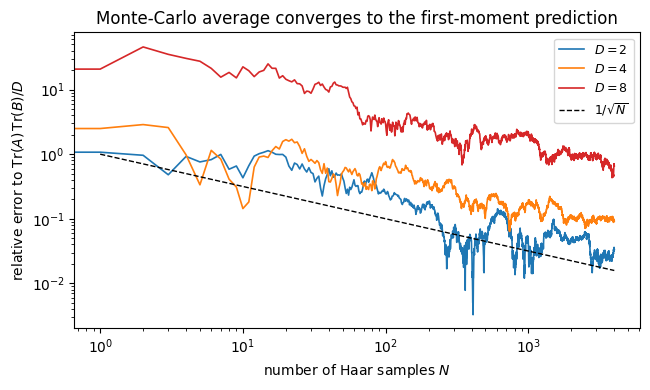
# --- Visualization: the Monte-Carlo Haar average converges to Tr(A)Tr(B)/D ---
import numpy as np
from scipy.stats import unitary_group
import matplotlib.pyplot as plt

rng = np.random.default_rng(0)
fig, ax = plt.subplots(figsize=(6.6, 4))
for D, c in zip([2, 4, 8], ["C0", "C1", "C3"]):
    A = rng.standard_normal((D, D)) + 1j * rng.standard_normal((D, D))
    B = rng.standard_normal((D, D)) + 1j * rng.standard_normal((D, D))
    pred = np.trace(A) * np.trace(B) / D
    Us = unitary_group.rvs(D, size=4000, random_state=rng)
    vals = np.array([np.trace(U @ A @ U.conj().T @ B) for U in Us])
    run = np.cumsum(vals) / np.arange(1, len(vals) + 1)      # running Haar average
    ax.plot(np.abs(run - pred) / max(abs(pred), 1e-9), color=c, lw=1.2, label=f"$D={D}$")
ax.plot(np.arange(1, 4001), 1.0 / np.sqrt(np.arange(1, 4001)), "k--", lw=1,
        label=r"$1/\sqrt{N}$")
ax.set_xscale("log"); ax.set_yscale("log")
ax.set_xlabel("number of Haar samples $N$")
ax.set_ylabel(r"relative error to $\mathrm{Tr}(A)\,\mathrm{Tr}(B)/D$")
ax.set_title("Monte-Carlo average converges to the first-moment prediction")
ax.legend(fontsize=9)

plt.tight_layout()
plt.show()

Takeaway

Haar-averaging a conjugated operator keeps only its trace, so \(\mathbb{E}_U[\mathrm{Tr}(U A U^\dagger B)] = \mathrm{Tr}(A)\,\mathrm{Tr}(B)/D\). All directional information in \(A\) and \(B\) is washed out, leaving a product of traces divided by the dimension.

Connections

This notebook computes the first Haar moment, the average of a single copy of a random unitary. Its second-moment partner, the twirl that sends an operator to a combination of the identity and the swap, is the single most reused calculation in the tutorial. It appears in the SWAP trick and the Page formula, then returns far from random states in the classical shadows channel, the randomized benchmarking decay, and the barren plateau variance. Recognizing it once means you have already done most of those later calculations.

References

• Collins, Moments and cumulants of polynomial random variables on unitary groups, the Itzykson-Zuber integral, and free probability, International Mathematics Research Notices (2003).
• Collins and Śniady, Integration with respect to the Haar measure on unitary, orthogonal and symplectic group, Communications in Mathematical Physics (2006).
• Collins et al., The Weingarten calculus, Notices of the American Mathematical Society (2022).
• Mele, Introduction to Haar Measure Tools in Quantum Information: A Beginner’s Tutorial, Quantum (2024). doi
• Płodzień, Information Scrambling, Quantum Chaos, and Haar-Random States, lecture notes (2025). arXiv:2511.14397