Classifying Quantum Phases with a Quantum Extreme Learning Machine
A standalone worked example. We take the ground state of a many-body Hamiltonian, push it once through a fixed quantum “reservoir”, read out a handful of low-weight Pauli expectation values, and train only a linear classifier on top. The classifier learns to tell the two phases of matter apart, and its decision boundary lands on the true quantum critical point, even though it was never shown an order parameter.
Motivation: phases, order parameters, and what a QELM changes
A quantum phase transition separates two qualitatively different ground states of a many-body system as a control parameter is tuned at zero temperature. The textbook way to detect one is to guess an order parameter: a specific observable (say, the magnetization) that is nonzero in one phase and vanishes in the other. Finding the right order parameter usually requires knowing the physics of the transition in advance.
A Quantum Extreme Learning Machine (QELM) turns this around. It is the one-shot, static cousin of a quantum reservoir computer:
The input is a quantum state, here the ground state \(|\psi_{\rm gs}(g)\rangle\).
A fixed, untrained quantum map (a scrambling unitary) spreads the input’s information across the whole register.
We measure a fixed bank of simple observables to get a feature vector.
Only a classical linear readout is trained.
The native advantage over classical machine learning is exactly step 1: the input can be a genuine quantum state, so no classical description (which would be exponentially large) is ever needed. The pedagogical punchline of this notebook: a generic scramble-then-measure feature map, with no knowledge of the order parameter, still separates the phases, and a linear readout on it crosses at the true critical point.
Problem statement
Model. The transverse-field Ising model (TFIM) on an open chain of \(N\) spins, \[
H(g) = -J\sum_{i} Z_i Z_{i+1} - g \sum_i X_i .
\] It has a quantum phase transition at \(g/J = 1\):
\(g > 1\): paramagnetic / disordered phase (the transverse field dominates).
Task. Given only the ground state at a field \(g\), decide which phase it is in.
Constraint. The classifier is trained on states drawn far from the critical point (clearly ordered or clearly disordered) and is never told the order parameter. We then test it on a dense sweep of \(g\) through the critical region and ask where its decision boundary falls.
QELM protocol (per input \(g\)). 1. Diagonalize \(H(g)\), take the ground state \(|\psi_{\rm gs}(g)\rangle\). 2. Evolve under a fixed nonintegrable scrambling unitary \(U = e^{-i H_{\rm res} t}\). 3. Read a fixed bank of low-weight Pauli expectation values \(f_\alpha = \langle \psi_{\rm gs}| U^\dagger O_\alpha U |\psi_{\rm gs}\rangle\). 4. Fit a linear (logistic) readout on \(f\) to predict the phase label.
Code
import numpy as npfrom scipy.linalg import expm, eighfrom sklearn.linear_model import LogisticRegressionfrom sklearn.preprocessing import StandardScalerfrom sklearn.decomposition import PCAimport matplotlib.pyplot as pltnp.set_printoptions(precision=3, suppress=True)I2 = np.eye(2, dtype=complex)X = np.array([[0, 1], [1, 0]], dtype=complex)Y = np.array([[0, -1j], [1j, 0]], dtype=complex)Z = np.array([[1, 0], [0, -1]], dtype=complex)def kron_op(single, site, N): op = np.array([[1.0]], dtype=complex)for j inrange(N): op = np.kron(op, single if j == site else I2)return op
The model Hamiltonian and its ground state
We build \(H(g)\) densely (for \(N=8\) the Hilbert space is only \(2^8 = 256\) dimensional) and take the lowest eigenvector. On an open chain the ground state is nondegenerate for \(g>0\), so this is unambiguous. Note the finite-size ground state is \(\mathbb{Z}_2\)-symmetric: the single-site magnetization \(\langle Z_i\rangle\) is zero in both phases, so it is useless as a naive order parameter here. The real signature of order lives in correlations\(\langle Z_i Z_j\rangle\), which the QELM never reads directly.
Code
def tfim_hamiltonian(N, J, g):"""H(g) = -J sum Z_i Z_{i+1} - g sum X_i on an open chain.""" H = np.zeros((2**N, 2**N), dtype=complex)for i inrange(N -1): H +=-J * (kron_op(Z, i, N) @ kron_op(Z, i +1, N))for i inrange(N): H +=-g * kron_op(X, i, N)return Hdef ground_state(N, J, g): w, v = eigh(tfim_hamiltonian(N, J, g))return v[:, 0].astype(complex)# Sanity check: <Z_0> = 0 in both phases (unbroken Z2), but the# nearest-neighbour correlation <Z_0 Z_1> is large when ordered, small when not.N =8; J =1.0for g in (0.3, 1.8): psi = ground_state(N, J, g) zz = np.vdot(psi, (kron_op(Z, 0, N) @ kron_op(Z, 1, N)) @ psi).real z0 = np.vdot(psi, kron_op(Z, 0, N) @ psi).realprint(f"g={g}: <Z0>={z0:+.3f} <Z0 Z1>={zz:+.3f}")
g=0.3: <Z0>=-0.000 <Z0 Z1>=+0.945
g=1.8: <Z0>=-0.000 <Z0 Z1>=+0.278
The fixed reservoir: a scrambling unitary
For the input state to be usefully re-expressed in low-weight observables, the reservoir must scramble: spread local information across the chain. A pure transverse-field Ising model is Jordan-Wigner integrable and does not scramble. Adding a longitudinal field \(h_z\) breaks integrability, so the mixed-field Ising Hamiltonian \[
H_{\rm res} = J_r \sum_i Z_i Z_{i+1} + h_x \sum_i X_i + h_z \sum_i Z_i
\] generates genuine scrambling dynamics. We fix its parameters and the evolution time \(t\)once; nothing in the reservoir is ever trained.
Code
def mixed_field_ising(N, Jr, hx, hz):"""Nonintegrable reservoir: Jr sum ZZ + hx sum X + hz sum Z.""" H = np.zeros((2**N, 2**N), dtype=complex)for i inrange(N -1): H += Jr * (kron_op(Z, i, N) @ kron_op(Z, i +1, N))for i inrange(N): H += hx * kron_op(X, i, N) + hz * kron_op(Z, i, N)return HJR, HX, HZ, T_EV =1.0, 1.05, 0.5, 2.5U = expm(-1j* mixed_field_ising(N, JR, HX, HZ) * T_EV) # fixed onceprint("scrambling unitary U:", U.shape, " unitary?", np.allclose(U.conj().T @ U, np.eye(2**N)))
scrambling unitary U: (256, 256) unitary? True
The fixed measurement bank
We read a bank of low-weight Pauli observables: all single-site \(\{X_i, Y_i, Z_i\}\) and nearest-neighbour \(\{X_iX_{i+1}, Y_iY_{i+1}, Z_iZ_{i+1}\}\). These are exactly the observables one can estimate cheaply on hardware. For a pure state \(\psi\), a Pauli string \(P = i^{p} X^{x} Z^{z}\) has \[
\langle P\rangle = \mathrm{Re}\sum_b \overline{\psi_b}\, W_b\, \psi_{b\oplus x},
\] an \(O(2^N)\) contraction we vectorize over the whole bank at once.
Code
_POP = np.array([bin(i).count('1') for i inrange(1<<16)])_PH = np.array([1, 1j, -1, -1j])def pauli_readout(N): bit =lambda i: 1<< (N -1- i) specs, names = [], []for i inrange(N): specs += [(bit(i), 0, 0), (bit(i), bit(i), 1), (0, bit(i), 0)] # X,Y,Z names += [f'X{i}', f'Y{i}', f'Z{i}']for i inrange(N -1): m = bit(i) | bit(i +1) specs += [(m, 0, 0), (m, m, 2), (0, m, 0)] # XX,YY,ZZ names += [f'X{i}X{i+1}', f'Y{i}Y{i+1}', f'Z{i}Z{i+1}'] b = np.arange(1<< N) COLS = np.array([b ^ x for (x, z, p) in specs]) W = np.array([_PH[p] * (1-2* (_POP[z & b] &1)) for (x, z, p) in specs], dtype=complex)return COLS, W, namesCOLS, W, names = pauli_readout(N)print(f"{len(names)} features, e.g. {names[:3]} ... {names[-3:]}")
45 features, e.g. ['X0', 'Y0', 'Z0'] ... ['X6X7', 'Y6Y7', 'Z6Z7']
The feature map
Putting it together: for each input \(g\) we form the ground state, evolve it once under the fixed \(U\), and read the bank. This is the entire “quantum” part of the learning machine, and none of it depends on the training labels.
Code
def qelm_features(psi_list, U, COLS, W):"""f_alpha = <psi| U^dag O_alpha U |psi>, evaluated on phi = U psi.""" F = np.zeros((len(psi_list), COLS.shape[0]))for n, psi inenumerate(psi_list): phi = U @ psi F[n] = np.real(np.conj(phi) * W * phi[COLS]).sum(axis=1)return F
Train far from criticality, test across the transition
We draw training fields only from the clearly-ordered (\(g \in [0.1, 0.65]\)) and clearly-disordered (\(g \in [1.35, 2.4]\)) windows, label them \(0\)/\(1\), and hold out a separate set of clear-region fields to report honest accuracy. The dense sweep \(g \in [0.02, 2.5]\) probes what the readout does in the critical region it never trained on.
The only trainable object is a logistic-regression readout on the standardized features. Because the features are linear in the density matrix\(\rho\), a linear readout is the well-posed choice: any expectation value the classifier needs is itself a linear functional of \(\rho\), so a linear combination of the measured features can reproduce it.
Visualize: feature-space geometry and the decision boundary
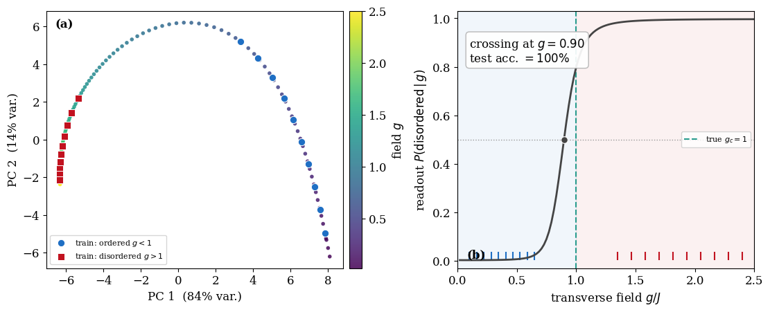
Panel (a) is a 2D PCA of the feature vectors. The ground states trace out a smooth one-dimensional manifold parametrized by \(g\); the ordered and disordered training states sit in clearly distinct regions, and the dense sweep threads between them. Panel (b) shows the trained readout’s predicted paramagnetic probability across the transition. The decision crossing \(P=\tfrac12\) lands right at the true critical point, purely from clear-region training data.
What happened. A fixed, untrained quantum scramble turned each ground state into a feature vector of ordinary low-weight expectation values. A linear readout, trained only on states far from the transition, learned the boundary between the two phases and placed it on the true critical point \(g_c = 1\). The QELM was never handed the magnetization or any correlation function to key on. The information distinguishing the phases is present in the ground state, and a generic scramble makes it linearly accessible in simple observables.
Why a linear readout is the right choice. Every feature is \(f_\alpha = \mathrm{Tr}(\rho\, U^\dagger O_\alpha U)\), a linear functional of the state \(\rho\). So any quantity that is itself linear in \(\rho\), including any other expectation value, is reachable by a linear combination of the features. The readout is well posed.
The caveat (a genuine limit). A quantity that is a nonlinear functional of \(\rho\) cannot be recovered this way. The entanglement entropy \(S = -\mathrm{Tr}(\rho_A \log \rho_A)\) is quadratic-and-worse in \(\rho\); no linear readout on single-copy expectation values can reproduce it, regardless of training. Detecting order through such nonlinear diagnostics requires multi-copy protocols (for example SWAP-test / shadow estimators), which is a different tool. The lesson: the QELM linearizes learning only for observables that are already linear in the state, and phase classification, luckily, is one of them.
Finite size. On an open chain of \(N=8\) the pseudo-critical point sits slightly below the thermodynamic \(g_c=1\), so the decision crossing appears near \(g\approx 0.9\). It sharpens toward \(g_c=1\) as \(N\) grows.