Barren Plateaus through the Lens of Quantum Fisher Information
This exercise connects the trainability of parameterized quantum circuits to the Quantum Fisher Information (QFI) with respect to variational parameters. The QFI stays \(\mathcal{O}(1)\) even for Haar-random circuits, so the state does move under the parameter; the barren plateau arises because the observable cannot detect that motion, a distinction the parameter-space geometry makes precise.
Background
The barren plateau is usually diagnosed from the gradient, but a vanishing gradient blends two separate facts. One is whether the quantum state actually changes when a parameter is varied. The other is whether the particular observable in the cost can detect that change. A flat gradient could mean the state is frozen, or it could mean the state is moving in a direction the measurement happens to be blind to, and the gradient on its own cannot tell these apart.
The quantum Fisher information pulls them apart. It measures how fast the state \(|\psi(\theta)\rangle\) moves through Hilbert space as \(\theta\) is tuned, counting distance with the natural geometry of quantum states, and it does so without reference to any observable. Up to a factor of four it equals the Fubini-Study metric, the standard way of measuring how far apart two nearby quantum states are, so a large quantum Fisher information means the state is genuinely sensitive to the parameter.
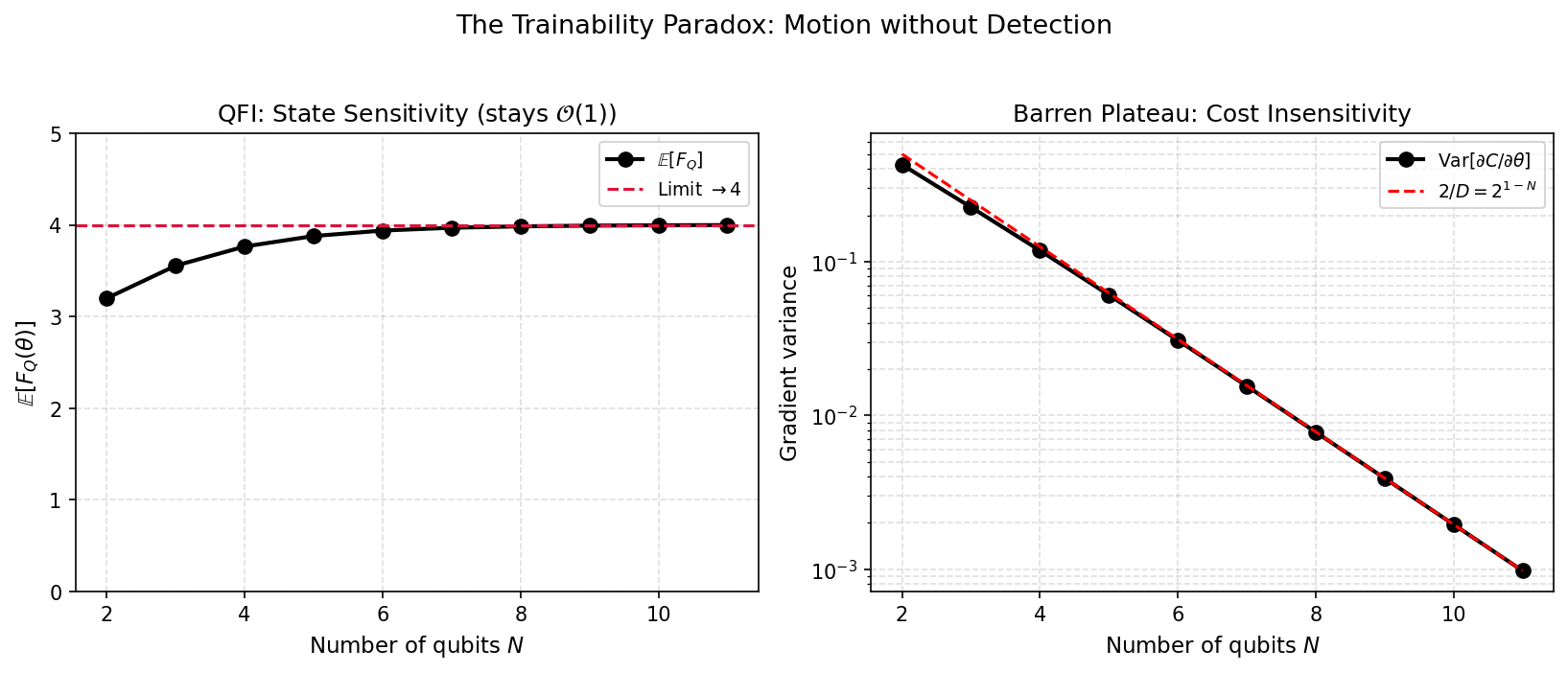
For a random circuit the two quantities point in opposite directions. The averaged quantum Fisher information of a traceless Pauli generator is \(4D/(D+1)\), which settles to \(4\) as \(D = 2^N\) grows, so the state stays fully responsive no matter how many qubits are added. The cost gradient over the same ensemble has variance of order \(1/D\), the familiar exponential collapse. The state slides a real distance along a geodesic of its space while the observable resolves only a tiny sliver of that motion, so almost all of the displacement lands outside what the cost can register.
The Cramér-Rao bound makes the contrast quantitative, setting the order-one Fisher information against the \(1/D\) gradient variance and locating the loss firmly in the readout. Reading the plateau this way shifts the blame from the geometry of the state to the observable, which is the reason local observables and ansätze built to point the cost along the directions the state explores can bring the slope back.
1. The Geometric Picture
Consider a parameterized circuit \(U(\boldsymbol{\theta})\) preparing the state \(|\psi(\boldsymbol{\theta})\rangle = U(\boldsymbol{\theta})|0\rangle\). The cost function is \(C(\boldsymbol{\theta}) = \langle \psi(\boldsymbol{\theta}) | O | \psi(\boldsymbol{\theta}) \rangle\) for some observable \(O\).
The Quantum Fisher Information (QFI) with respect to the parameter \(\theta_k\) measures how sensitively the quantum state responds to infinitesimal changes in \(\theta_k\):
This is precisely four times the Fubini-Study metric\(g_{kk}^{\mathrm{FS}}\) on the projective Hilbert space \(\mathbb{CP}^{D-1}\):
\[
F_Q(\theta_k) = 4\, g_{kk}^{\mathrm{FS}}.
\]
When \(F_Q(\theta_k) \to 0\), the state \(|\psi\rangle\) becomes insensitive to \(\theta_k\): an infinitesimal change in \(\theta_k\) produces a negligible change in the quantum state. If the state doesn’t change, the cost function doesn’t change, and the gradient vanishes.
This provides a purely geometric, observable-independent explanation of barren plateaus: the parameter landscape becomes metrically flat in the Fubini-Study sense.
2. Mathematical Toolbox
Tool 1, QFI for pure states: For \(|\psi(\theta)\rangle = e^{-i\theta G} |\psi_0\rangle\) with generator \(G\), \[
F_Q(\theta) = 4\, \mathrm{Var}_{|\psi_0\rangle}(G) = 4\left(\langle G^2 \rangle - \langle G \rangle^2\right).
\]
Tool 2, Cramér-Rao bound on gradients: The variance of \(\partial C / \partial \theta_k\) over the parameter distribution is bounded by: \[
\mathrm{Var}\!\left[\frac{\partial C}{\partial \theta_k}\right] \leq \|O\|^2 \cdot F_Q(\theta_k).
\] If \(F_Q \to 0\), the gradient is forced to vanish regardless of the observable \(O\).
Tool 3, Haar first moment (Weingarten \(k=1\)):\[
\mathbb{E}_{U}[U^\dagger A\, U] = \frac{\mathrm{Tr}(A)}{D}\, I.
\]
Tool 4, Haar second moment (Weingarten \(k=2\)):\[
\mathbb{E}_{U}[U^\dagger A\, U \otimes U^\dagger B\, U] = \alpha(A,B)\, I \otimes I + \beta(A,B)\, \mathrm{SWAP},
\] where \(\alpha = \frac{D\,\mathrm{Tr}(A)\mathrm{Tr}(B) - \mathrm{Tr}(AB)}{D(D^2-1)}\) and \(\beta = \frac{D\,\mathrm{Tr}(AB) - \mathrm{Tr}(A)\mathrm{Tr}(B)}{D(D^2-1)}\).
3. Exercise
Consider a circuit \(U(\theta) = V_2\, e^{-i\theta G}\, V_1\) where \(V_1, V_2\) are Haar-random and \(G\) is a fixed Hermitian generator (e.g. a single Pauli).
(a) Show that the QFI with respect to \(\theta\) is \(F_Q(\theta) = 4\,\mathrm{Var}_{|\psi_1\rangle}(G)\) where \(|\psi_1\rangle = V_1|0\rangle\).
(b) Show that for Haar-random \(V_1\), the expected QFI is: \[
\mathbb{E}_{V_1}[F_Q] = \frac{4}{D+1}\left(\mathrm{Tr}(G^2) - \frac{(\mathrm{Tr}\, G)^2}{D}\right).
\]
(c) For a traceless Pauli generator \(G\) with \(G^2 = I\) and \(\mathrm{Tr}(G) = 0\), show that \(\mathbb{E}[F_Q] = \frac{4D}{D+1} \xrightarrow{D \to \infty} 4\). Compare this with the gradient variance \(\sim 1/D\).
(d) Using the pointwise bound \(|\partial_\theta C|^2 \leq F_Q\,\mathrm{Var}_\psi(O)\), show that the QFI alone bounds the gradient only by \(\mathcal{O}(1)\). Then explain why the ensemble variance is nonetheless \(\mathrm{Var}[\partial_\theta C] \sim 2/D\), and reconcile the two statements.
4. Step-by-Step Derivation
Part (a): QFI from the variance of the generator
At \(\theta = 0\), the state is \(|\psi_1\rangle = V_1|0\rangle\) and the parameter acts via \(e^{-i\theta G}\). The QFI formula for pure states gives:
Note: the post-rotation \(V_2\) does not affect \(F_Q\) because the Fubini-Study metric is invariant under global unitaries. The QFI captures the intrinsic sensitivity of the state manifold, not the measurement basis.
Part (b): Haar-averaged QFI
We need \(\mathbb{E}_{V_1}[\langle\psi_1|G^2|\psi_1\rangle]\) and \(\mathbb{E}_{V_1}[\langle\psi_1|G|\psi_1\rangle^2]\).
First term (using Tool 3, \(k=1\)): \[
\mathbb{E}[\langle G^2 \rangle] = \mathrm{Tr}\!\left(\frac{I}{D} G^2\right) = \frac{\mathrm{Tr}(G^2)}{D}.
\]
Second term (using Tool 4, \(k=2\)): Since \(\langle G \rangle^2 = \langle \psi_1 | G | \psi_1 \rangle^2\), this is a second-moment integral: \[
\mathbb{E}[\langle G \rangle^2] = \frac{\mathrm{Tr}(G)^2 + \mathrm{Tr}(G^2)}{D(D+1)}.
\]
This is an \(\mathcal{O}(1)\) constant. The QFI does not vanish exponentially. The quantum state is sensitive to the parameter \(\theta\).
But recall that the gradient variance \(\mathrm{Var}[\partial C / \partial \theta] \sim 1/D \to 0\) exponentially. This sits in apparent tension with the QFI: the state moves in Hilbert space, yet the cost barely changes.
Resolution: The state \(|\psi(\theta)\rangle\) moves along a geodesic in \(\mathbb{CP}^{D-1}\), but the observable \(O\) projects onto a tiny subspace. The motion is “perpendicular” to the cost landscape. The QFI tells us the state moves; the barren plateau tells us it moves in a direction that doesn’t matter for the observable. This is the curse of expressibility: the circuit explores exponentially many directions, but only \(\mathcal{O}(1)\) of them align with a given cost function.
Part (d): What the QFI bound does and does not give
The gradient is \(\partial_\theta C = 2\,\mathrm{Im}\langle \psi | O | \partial_\theta \psi \rangle\). Cauchy-Schwarz together with the QFI gives the pointwise bound
For a single Pauli on a Haar-random state both factors are \(\mathcal{O}(1)\). Part (c) gave \(F_Q \to 4\), while \(\mathrm{Var}_\psi(O) \approx 1\) since \(\langle O^2\rangle = 1\) and \(\langle O\rangle^2 \sim 1/D\). The QFI bound on its own therefore only certifies \(|\partial_\theta C| = \mathcal{O}(1)\) and does not produce the barren plateau.
The exponential suppression lives in the ensemble, not in this single-point bound. Averaging \(|\partial_\theta C|^2\) over Haar-random \(V_1, V_2\) with the \(k=2\) Weingarten formula gives
because the direction in which the state actually moves with \(\theta\) is generically almost orthogonal to the one the observable \(O\) resolves. The QFI says the state moves; the Weingarten average says the cost barely registers it.
5. Physical Interpretation: Geometry vs Trainability
The QFI analysis decomposes the barren plateau into three quantities:
Quantity
Scaling
Meaning
\(F_Q(\theta)\)
\(\mathcal{O}(1)\)
The state does move in Hilbert space
\(\mathrm{Var}_{|\psi\rangle}(O)\)
\(\mathcal{O}(1/D)\)
The observable cannot distinguish nearby states
\(\mathrm{Var}[\partial C/\partial\theta]\)
\(\mathcal{O}(1/D)\)
The cost landscape is flat
The barren plateau is not a failure of the parameterization to move the state, it is a failure of the observable to detect the motion. The Fubini-Study geodesic ball explored by the parameter \(\theta\) has an exponentially large volume, but the “shadow” of this ball onto the cost function is exponentially thin.
This motivates two strategies: 1. Local observables: If \(O\) acts on \(k\) qubits, \(\mathrm{Tr}(O^2) \sim 2^k\) and \(\mathrm{Var}[\partial C] \sim 2^k / D\), which is polynomial for \(k = \mathcal{O}(\log N)\). 2. Structured ans"atze: Restrict the circuit to a low-dimensional submanifold of \(\mathbb{CP}^{D-1}\) where \(F_Q\) and the cost function are aligned.
E[F_Q] = 4*(D*TrG2 - TrG**2)/(D*(D + 1))
Verified: E[F_Q] = 4/(D+1) * (Tr(G^2) - Tr(G)^2/D)

Pauli generator: E[F_Q] = 4*D/(D + 1)
Large D limit: 4

Gradient variance bound: 4*TrO2/(D + 1)
Large D: ~ 0 * Tr(O^2) / D
7. Numerical Verification (NumPy)
Code
import numpy as npfrom scipy.stats import unitary_groupnp.random.seed(42)X = np.array([[0, 1], [1, 0]], dtype=complex)Z = np.array([[1, 0], [0, -1]], dtype=complex)def pauli_on_qubit1(op, N):"""op acting on qubit 1, identity on the remaining N-1 qubits.""" M = opfor _ inrange(N -1): M = np.kron(M, np.eye(2))return Mprint('QFI Concentration for Haar-Random States')print('='*66)print(f'{"N":>3s}{"D":>5s}{"E[F_Q] MC":>10s}{"4D/(D+1)":>10s}{"Var[dC] MC":>11s}{"~2/D":>9s}')print('-'*66)for N in [2, 3, 4, 5, 6]: D =2**N# Generator: Z on qubit 1 (traceless Pauli, G^2 = I) G = pauli_on_qubit1(Z, N)# Observable: X on qubit 1 - does NOT commute with G, so the gradient# 2*Im<psi|O~ G|psi> is generically nonzero. A Haar post-rotation V2# conjugates O (O~ = V2^dagger O V2), implementing U(theta)=V2 e^{-i theta G} V1. O = pauli_on_qubit1(X, N) fq_list = [] grad_list = []for _ inrange(3000): V1 = unitary_group.rvs(D) V2 = unitary_group.rvs(D) psi = V1[:, 0]# QFI = 4 * Var(G) eG = (psi.conj() @ G @ psi).real eG2 = (psi.conj() @ G @ G @ psi).real fq =4* (eG2 - eG**2) fq_list.append(fq)# Gradient at theta=0: dC/dtheta = i<psi|[G, O~]|psi> = 2 Im<psi|O~ G|psi> O_tilde = V2.conj().T @ O @ V2 grad =2* np.imag(psi.conj() @ O_tilde @ G @ psi) grad_list.append(grad) mc_fq = np.mean(fq_list) th_fq =4* D / (D +1) mc_var = np.var(grad_list)# Exact gradient variance for this single-Pauli setup (Tr O^2 = D):# Var[dC] = 2 D^2 / ((D-1)(D+1)^2) -> ~ 2/D as D -> infinity. th_var =2* D**2/ ((D -1) * (D +1)**2)print(f'{N:3d}{D:5d}{mc_fq:10.4f}{th_fq:10.4f}{mc_var:11.6f}{th_var:9.6f}')assertabs(mc_fq - th_fq) <0.2assert mc_var >0# gradient is genuinely nonzeroassertabs(mc_var - th_var) / th_var <0.25# scales as ~1/Dprint('\nKey insight: F_Q ~ O(1) but Var[grad] ~ O(1/D)!')print('The state moves, but the cost can barely detect the motion.')
QFI Concentration for Haar-Random States
==================================================================
  N      D   E[F_Q] MC    4D/(D+1)   Var[dC] MC       ~2/D
------------------------------------------------------------------
2 4 3.1903 3.2000 0.445567 0.426667
3 8 3.5452 3.5556 0.215734 0.225750
4 16 3.7645 3.7647 0.120488 0.118108
5 32 3.8807 3.8788 0.060531 0.060665
  6     64      3.9420      3.9385     0.030338   0.030777

Key insight: F_Q ~ O(1) but Var[grad] ~ O(1/D)!
The state moves, but the cost can barely detect the motion.
8. Visual Proof: QFI vs Gradient Scaling
Takeaway
For a traceless Pauli generator the expected QFI tends to \(4\) as \(D\to\infty\), so the state stays sensitive to the parameter even as the cost gradient vanishes as \(1/D\). The observable resolves only an \(O(1)\)-dimensional slice of the motion, and recovering trainability means aligning it with the directions the circuit explores through local observables or structured ansätze.
This is the barren plateau viewed through the quantum Fisher information, which separates whether the state moves under a parameter from whether the cost can detect that motion. The gradient collapse is the same Haar second moment as in the barren plateau notebook. The metrological side of the same quantity drives the GHZ fragility in the applications part.
References
McClean et al., Barren plateaus in quantum neural network training landscapes, Nature Communications (2018).
Stokes et al., Quantum Natural Gradient, Quantum (2020).
Braunstein and Caves, Statistical distance and the geometry of quantum states, Physical Review Letters (1994).
Płodzień, Information Scrambling, Quantum Chaos, and Haar-Random States, lecture notes (2025). arXiv:2511.14397