Quantum Extreme Learning Machines and the XOR Problem
This notebook is self-contained. It builds a quantum extreme learning machine (QELM) that solves the classic XOR classification problem, and isolates the role of the fixed quantum dynamics through a raw-vs-QELM ablation.
The QELM idea. A quantum extreme learning machine keeps training trivial and lets the physics do the hard part. Classical data is written into a fixed quantum state, that state is pushed through a fixed, untrained scrambling unitary, and a bank of local observables is measured. Only a linear readout on those measured expectation values is fit. The quantum dynamics supply the nonlinearity; the learning step stays a plain linear model.
Motivation: XOR is not linearly separable
The XOR (exclusive-or) problem is the textbook example of a task a linear model cannot solve. In its continuous form the two input coordinates \((x_1, x_2)\) carry the label \[
y = \mathrm{sign}(x_1 x_2),
\] so the positive class occupies the two quadrants where \(x_1\) and \(x_2\) share a sign, and the negative class occupies the other two. The classes interlock in a checkerboard. No straight line separates a checkerboard, so a linear classifier on the raw inputs \((x_1, x_2)\) is stuck at chance.
The feature-map fix. A linear model fails only in the raw coordinates. If we first map each input through a fixed nonlinear feature map \(x \mapsto f(x)\) into a higher-dimensional feature space, a task that was not linearly separable can become linearly separable there. Learning then reduces to fitting a hyperplane in feature space, which is a linear problem again. The whole difficulty moves into the choice of feature map.
The quantum feature map. A QELM realizes the feature map with quantum dynamics. We angle-encode \((x_1, x_2)\) into a small qubit register, evolve under one fixed nonintegrable Hamiltonian, and read a set of low-weight Pauli expectation values. The scrambling dynamics mix the two coordinates into every qubit, so single-qubit observables become genuinely two-coordinate nonlinear functions, including the \(x_1 x_2\) product that XOR needs. None of this pipeline is trained: only the final linear readout is.
Problem statement
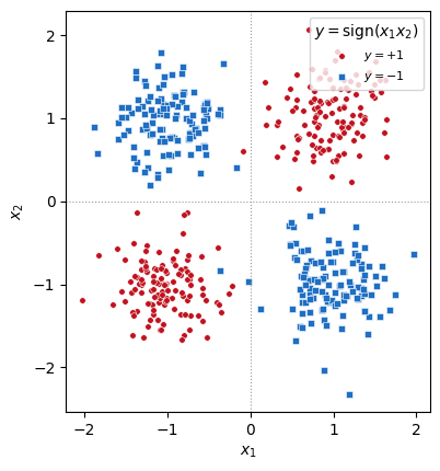
Sample a continuous XOR dataset: four Gaussian clusters near \((\pm 1, \pm 1)\), labelled \(y = \mathrm{sign}(x_1 x_2)\).
Fix a quantum feature map: angle-encode \((x_1, x_2)\) into \(N=4\) qubits, apply a fixed scrambling unitary \(U = e^{-i H t}\) with \(H\) the nonintegrable mixed-field Ising chain, and read the weight-one Pauli bank \(\{\langle X_i\rangle, \langle Y_i\rangle, \langle Z_i\rangle\}\).
Train a single linear classifier (logistic regression) three ways and compare:
on the raw inputs \((x_1, x_2)\);
on the Pauli features of the bare (unscrambled) encoded state;
on the Pauli features after the fixed scrambling \(U\) (the QELM).
The expected outcome: raw \(\approx 50\%\), bare \(\approx 50\%\), QELM \(\approx 100\%\).
Four isotropic Gaussian clusters, one per quadrant, with label \(y=\mathrm{sign}(x_1 x_2)\). The clusters on the main diagonal are one class; the clusters on the anti-diagonal are the other. This is the continuous XOR / checkerboard.
A straight line can peel off at most one cluster from the rest, never the two diagonal clusters together. This is the non-separability we have to defeat.
The quantum feature map
Encoding. We use \(N=4\) qubits. Qubits \(0,1\) carry \(x_1\) and qubits \(2,3\) carry \(x_2\), each through a single-qubit rotation \[
R_y(\alpha x)\,|0\rangle = \cos\tfrac{\alpha x}{2}\,|0\rangle
+ \sin\tfrac{\alpha x}{2}\,|1\rangle .
\] On this product state a single-qubit measurement gives \(\langle Z\rangle=\cos(\alpha x)\), \(\langle X\rangle=\sin(\alpha x)\), \(\langle Y\rangle=0\), all functions of one coordinate. The bare encoded state therefore has no \(x_1 x_2\) cross term to read out from any single qubit.
Scrambling. The fixed feature map is one step of evolution under the nonintegrable mixed-field Ising Hamiltonian \[
H = J\sum_i Z_i Z_{i+1} + h_x\sum_i X_i + h_z\sum_i Z_i .
\] The longitudinal field \(h_z\) breaks the Jordan-Wigner integrability of the pure transverse-field model, so \(U = e^{-i H t}\) scrambles: it entangles the qubits and spreads each encoded coordinate over the whole register. After \(U\), a single-qubit observable \(\langle Z_i\rangle\) is a function of both\(x_1\) and \(x_2\), and its Taylor expansion contains the product \(x_1 x_2\). That product is exactly the feature XOR requires.
Readout. We measure the weight-one Pauli bank \(\{\langle X_i\rangle, \langle Y_i\rangle, \langle Z_i\rangle\}_{i=0}^{N-1}\), giving a \(3N=12\)-dimensional feature vector \(f(x_1, x_2)\).
Code
I2 = np.eye(2, dtype=complex)X = np.array([[0, 1], [1, 0]], dtype=complex)Y = np.array([[0, -1j], [1j, 0]], dtype=complex)Z = np.array([[1, 0], [0, -1]], dtype=complex)def kron_op(single, site, N): op = np.array([[1.0]], dtype=complex)for j inrange(N): op = np.kron(op, single if j == site else I2)return opdef mixed_field_ising(N, J, hx, hz): H = np.zeros((2** N, 2** N), dtype=complex)for i inrange(N -1): H += J * (kron_op(Z, i, N) @ kron_op(Z, i +1, N))for i inrange(N): H += hx * kron_op(X, i, N) + hz * kron_op(Z, i, N)return HQUBIT_COORD = [0, 0, 1, 1] # qubits 0,1 -> x1 ; qubits 2,3 -> x2def encode(x1, x2, N, alpha): coords = (x1, x2) psi = np.array([1.0], dtype=complex)for j inrange(N): th = alpha * coords[QUBIT_COORD[j]] psi = np.kron(psi, np.array([np.cos(th /2), np.sin(th /2)], dtype=complex))return psi
The Pauli bank is precomputed as index/weight arrays: for a pure state \(\psi\), a Pauli \(P = i^{p} X^{x} Z^{z}\) has \(\langle P\rangle = \mathrm{Re}\sum_b \overline{\psi_b}\, W_b\, \psi_{b\oplus x}\), an \(O(2^N)\) contraction. We check it against the brute-force \(\langle\psi|P|\psi\rangle\).
Code
_POP = np.array([bin(i).count("1") for i inrange(1<<16)])_PH = np.array([1, 1j, -1, -1j])def pauli_readout(N): bit =lambda i: 1<< (N -1- i) specs, names = [], []for i inrange(N): specs += [(bit(i), 0, 0), (bit(i), bit(i), 1), (0, bit(i), 0)] # X, Y, Z names += [f"X{i}", f"Y{i}", f"Z{i}"] b = np.arange(1<< N) COLS = np.array([b ^ x for (x, z, p) in specs]) W = np.array([_PH[p] * (1-2* (_POP[z & b] &1)) for (x, z, p) in specs], dtype=complex)return COLS, W, names# sanity check the fast readout against brute forceN =4COLS, W, names = pauli_readout(N)psi = encode(0.7, -1.1, N, 1.0)fast = np.real(np.conj(psi) * W * psi[COLS]).sum(axis=1)brute = [np.real(psi.conj() @ (kron_op({'X': X, 'Y': Y, 'Z': Z}[nm[0]], int(nm[1]), N) @ psi))for nm in names]print("max |fast - brute| =", np.max(np.abs(fast - np.array(brute))))
max |fast - brute| = 1.1102230246251565e-16
Code
def qelm_features(XY, N, U, COLS, W, alpha): F = np.zeros((len(XY), COLS.shape[0]))for n, (x1, x2) inenumerate(XY): psi = encode(x1, x2, N, alpha)if U isnotNone: psi = U @ psi F[n] = np.real(np.conj(psi) * W * psi[COLS]).sum(axis=1)return FJ, HX, HZ =1.0, 0.9, 0.8# nonintegrable mixed-field Ising scramblerT_EV =2.0# fixed scrambling time (untrained)ALPHA =1.0# angle-encoding scaleH = mixed_field_ising(N, J, HX, HZ)U = expm(-1j* H * T_EV) # the fixed, untrained feature-map unitaryprint("U is unitary:", np.allclose(U.conj().T @ U, np.eye(2** N)))
U is unitary: True
The ablation
The same logistic-regression classifier is fit three ways. Only the input features change: raw coordinates, bare-encoding Pauli features, and QELM Pauli features. The quantum pipeline is never trained; only the linear readout weights are.
Code
def fit_score(F_tr, y_tr, F_te, y_te, C=10.0): clf = LogisticRegression(max_iter=5000, C=C).fit(F_tr, y_tr)return clf, float(clf.score(F_te, y_te))# (1) raw inputsraw_clf, acc_raw = fit_score(XY_tr, y_tr, XY_te, y_te)# (2) bare encoding, no scrambling (U = None)Fb_tr = qelm_features(XY_tr, N, None, COLS, W, ALPHA)Fb_te = qelm_features(XY_te, N, None, COLS, W, ALPHA)_, acc_bare = fit_score(Fb_tr, y_tr, Fb_te, y_te)# (3) QELM: same features after the fixed scrambling UFs_tr = qelm_features(XY_tr, N, U, COLS, W, ALPHA)Fs_te = qelm_features(XY_te, N, U, COLS, W, ALPHA)qelm_clf, acc_qelm = fit_score(Fs_tr, y_tr, Fs_te, y_te)print(f"raw-linear test accuracy = {acc_raw:.3f}")print(f"bare-encode test accuracy = {acc_bare:.3f} (no scrambling)")print(f"QELM test accuracy = {acc_qelm:.3f}")
raw-linear   test accuracy = 0.453
bare-encode  test accuracy = 0.500   (no scrambling)
QELM         test accuracy = 0.979
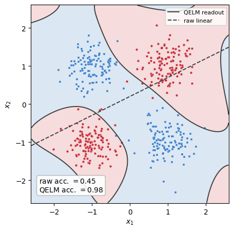
The raw linear model sits at chance: XOR is not linearly separable. The bare encoding does no better, because every weight-one Pauli of the unscrambled product state depends on a single coordinate, so the features are additive across \(x_1\) and \(x_2\) and a linear readout of them still cannot form the product. Turning on the fixed scrambling \(U\) lifts the accuracy to near \(100\%\): the dynamics, not the readout, supply the \(x_1 x_2\) feature. The scrambling is doing the learning-relevant work.
Decision regions
We evaluate the trained QELM readout on a dense grid to see the decision regions it carves in the \((x_1, x_2)\) plane, and overlay the raw linear boundary, which can only be a straight line.
The QELM readout wraps its decision boundary around all four clusters and recovers the checkerboard, while the raw linear model is confined to a single straight cut that gets XOR half right. The fixed quantum feature map made a non-separable problem linearly separable, and the ablation pins the credit precisely: with the same encoding and the same linear readout, it is the fixed scrambling unitary that supplies the nonlinear \(x_1 x_2\) feature. This is the QELM at its cleanest, the physics learns the representation, and only a hyperplane is fit on top.