Haar Measure & Weingarten Calculus, numerical solution.
The Asymptotic Page Formula via Marchenko-Pastur
Background
Take a pure state of a bipartite system and trace out one part to obtain the reduced state of the other. Its entanglement entropy measures how mixed that reduction is, and therefore how entangled the two parts are across the cut. The Page formula answers what this entropy looks like on average when the global state is drawn at random from the Haar measure, for a subsystem of dimension \(m\) sitting inside a complement of dimension \(n\) with \(m \le n\).
The answer is that the mean entropy lies just below the largest value it could take. The maximum is \(\ln m\), reached when the reduction is exactly maximally mixed, and the average falls short of it by a small deficit. In the regime studied here that deficit is \(m/(2n)\), so the entropy approaches \(\ln m - m/(2n)\). When the complement is much larger than the subsystem the correction is tiny and a typical reduction is nearly maximally mixed.
The derivation rests on the spectrum of the random reduced state, whose rescaled eigenvalues follow the Marchenko-Pastur distribution familiar from random matrix theory. Averaging the entropy function against this spectral law, and expanding around the mean eigenvalue, produces the logarithm plus the correction in a couple of clean steps. The variance of that distribution is what sets the size of the deficit.
This result is a cornerstone of the typicality arguments that run through random states and scrambling dynamics, where Haar-random states model thermalized ones. The size of the deficit is also what distinguishes a generic random state, slightly short of maximal, from one whose reduction is exactly maximally mixed. The notebook reproduces both the exact Page value and its asymptotic form by sampling random states.
Mathematical background
The exact average follows from the eigenvalue statistics of \(\rho_A\). Writing the Haar-random state in a product basis and tracing out \(B\) gives \(\rho_A = W/\mathrm{Tr}\,W\) with \(W = XX^\dagger\) a complex Wishart matrix built from an \(m \times n\) Gaussian matrix \(X\). The joint density of the eigenvalues \(\{\lambda_i\}\) of \(\rho_A\) is
The factor \(\prod_{i<j}(\lambda_i-\lambda_j)^2\) is the level repulsion of the unitary (\(\beta = 2\)) ensemble, and the delta function fixes the unit trace. Averaging the von Neumann entropy \(S(\rho_A) = -\sum_i \lambda_i \ln \lambda_i\) over this density gives Page’s exact result for \(m \le n\),
whose large-dimension expansion is \(\mathbb{E}[S] \simeq \ln m - \tfrac{m}{2n}\). The same density yields the average purity \(\mathbb{E}[\mathrm{Tr}\,\rho_A^2] = (m+n)/(mn+1)\), which tends to \(1/m\) as the environment grows. The Marchenko-Pastur law used below is the continuum limit of this eigenvalue density when \(m, n \to \infty\) at fixed ratio \(c = m/n\), so the two routes to the Page value describe the same statistics at different resolutions.
Motivation
Page’s formula gives the average entanglement entropy of a subsystem in a Haar-random state. It connects random-state geometry to quantum information by showing that typical states are nearly maximally entangled. The asymptotic form \(\mathbb{E}[S] \approx \ln m - m/(2n)\) (valid for \(m \leq n\)) combines two ingredients: (1) the eigenvalues of a random reduced state follow the Marchenko-Pastur distribution, and (2) the entropy correction follows from a short Taylor expansion.
Exercise
Derive the asymptotic Page formula
\[
\mathbb{E}[S(\rho_A)] \approx \ln m - \frac{m}{2n}
\]
by treating the eigenvalues of \(\rho_A\) as following the Marchenko-Pastur law with ratio \(c = m/n\).
Solution
Step 1: Setup
The \(m\) eigenvalues \(\lambda_j\) of \(\rho_A\) satisfy \(\sum_j \lambda_j = 1\) and \(\lambda_j \geq 0\). Introduce rescaled variables \(x_j = m\lambda_j\) so that \(\langle x \rangle = 1\). The entropy is:
\[
S = -\sum_j \lambda_j \ln \lambda_j = -\sum_j \frac{x_j}{m} \ln\frac{x_j}{m} = \ln m - \frac{1}{m}\sum_j x_j \ln x_j.
\]
In the large-\(m\) limit, the empirical spectral distribution of the \(x_j\) converges to the Marchenko-Pastur law with parameter \(c = m/n\).
Step 2: Taylor expansion
Define \(f(x) = x\ln x\). Taylor-expand around the mean \(x = 1\):
(The variance of the Marchenko-Pastur distribution with mean 1 and ratio \(c\) is exactly \(c\).)
Substituting back:
\[
\mathbb{E}[S] = \ln m - \frac{1}{m} \cdot m \cdot \frac{m}{2n} = \ln m - \frac{m}{2n}.
\]
\[
\boxed{\mathbb{E}[S(\rho_A)] \approx \ln m - \frac{m}{2n}.}
\]
Physical interpretation: The leading term \(\ln m\) is the maximal entanglement entropy, a random state is nearly maximally entangled. The correction \(-m/(2n)\) quantifies the small deficit and vanishes when \(n \gg m\) (the complement is much larger than the subsystem).
Symbolic Verification (SymPy)
Code
import sympy as spfrom sympy import harmonic, Rational, Symbol, simplify, logd_A = Symbol('d_A', positive=True, integer=True)d_B = Symbol('d_B', positive=True, integer=True)# Page formula: E[S_A] = sum_{k=d_B+1}^{d_A*d_B} 1/k - (d_A-1)/(2*d_B)# For d_A <= d_B# Approximate: E[S_A] ~ log(d_A) - d_A/(2*d_B)print('Page formula for entanglement entropy:')print(' E[S_A] = H(d_A*d_B) - H(d_B) - (d_A - 1)/(2*d_B)')print(' where H(n) = sum_{k=1}^{n} 1/k is the harmonic number')print()# Numerical check for small subsystemsimport numpy as npfor da in [2, 4]:for db in [4, 8, 16]:if da > db: continue# Exact Page formula S =sum(1/k for k inrange(db+1, da*db+1)) - (da-1)/(2*db) S_approx = np.log(da) - da/(2*db)print(f' d_A={da}, d_B={db}: S_exact={S:.4f}, S_approx={S_approx:.4f}, log(d_A)={np.log(da):.4f}')
Page formula for entanglement entropy:
  E[S_A] = H(d_A*d_B) - H(d_B) - (d_A - 1)/(2*d_B)
  where H(n) = sum_{k=1}^{n} 1/k is the harmonic number

  d_A=2, d_B=4: S_exact=0.5095, S_approx=0.4431, log(d_A)=0.6931
  d_A=2, d_B=8: S_exact=0.6004, S_approx=0.5681, log(d_A)=0.6931
  d_A=2, d_B=16: S_exact=0.6465, S_approx=0.6306, log(d_A)=0.6931
  d_A=4, d_B=4: S_exact=0.9224, S_approx=0.8863, log(d_A)=1.3863
  d_A=4, d_B=8: S_exact=1.1531, S_approx=1.1363, log(d_A)=1.3863
  d_A=4, d_B=16: S_exact=1.2694, S_approx=1.2613, log(d_A)=1.3863
Numerical Verification
Code
import numpy as npfrom scipy.stats import unitary_groupnp.random.seed(42)print(f"{'(m,n)':>8s}{'E[S] (MC)':>10s}{'ln(m)−m/2n':>12s}{'error':>8s}")print(f"{'─'*8:>8s}{'─'*10:>10s}{'─'*12:>12s}{'─'*8:>8s}")for m, n in [(2,2), (4,4), (8,8), (16,16), (4,16), (8,64)]: D = m * n n_samples =min(10000, max(1000, 200000//D)) entropies = []for _ inrange(n_samples): psi = unitary_group.rvs(D)[:, 0] rho = np.outer(psi, psi.conj()).reshape(m, n, m, n) rho_A = np.trace(rho, axis1=1, axis2=3) eigs = np.linalg.eigvalsh(rho_A) eigs = eigs[eigs >1e-15] S =-np.sum(eigs * np.log(eigs)) entropies.append(S) E_S = np.mean(entropies) S_page = np.log(m) - m/(2*n) err =abs(E_S - S_page)print(f"({m},{n}){' '*(6-len(str(m))-len(str(n)))}{E_S:10.4f}{S_page:12.4f}{err:8.4f}")print("\nPage formula confirmed: E[S] → ln(m) − m/(2n).")
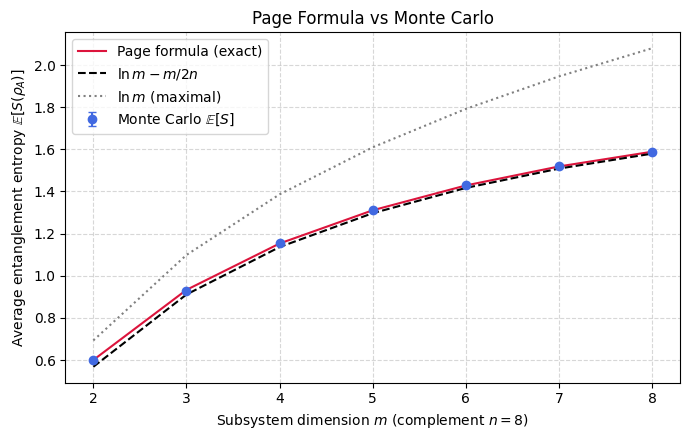
%matplotlib inlineimport numpy as npimport matplotlib.pyplot as pltfrom scipy.stats import unitary_groupnp.random.seed(0)# Fix the complement dimension n; vary the subsystem dimension m.n =8ms = np.arange(2, 9)n_samples =1200mc_mean, mc_err = [], []for m in ms: D = m * n S_list = np.empty(n_samples)for s inrange(n_samples): psi = unitary_group.rvs(D)[:, 0] rho_A = psi.reshape(m, n) @ psi.reshape(m, n).conj().T ev = np.linalg.eigvalsh(rho_A) ev = ev[ev >1e-15] S_list[s] =-np.sum(ev * np.log(ev)) mc_mean.append(S_list.mean()) mc_err.append(S_list.std() / np.sqrt(n_samples))def page_exact(m, n): D = m * nreturnsum(1.0/ k for k inrange(n +1, D +1)) - (m -1) / (2.0* n)page_vals = [page_exact(m, n) for m in ms]asymp = np.log(ms) - ms / (2.0* n)plt.figure(figsize=(7, 4.5))plt.errorbar(ms, mc_mean, yerr=mc_err, fmt='o', color='royalblue', capsize=3, label='Monte Carlo $\\mathbb{E}[S]$')plt.plot(ms, page_vals, '-', color='crimson', label='Page formula (exact)')plt.plot(ms, asymp, '--', color='black', label=r'$\ln m - m/2n$')plt.plot(ms, np.log(ms), ':', color='gray', label=r'$\ln m$ (maximal)')plt.xlabel(r"Subsystem dimension $m$ (complement $n=8$)")plt.ylabel(r"Average entanglement entropy $\mathbb{E}[S(\rho_A)]$")plt.title("Page Formula vs Monte Carlo")plt.legend()plt.grid(True, ls="--", alpha=0.5)plt.tight_layout()plt.show()
Takeaway
The average entanglement entropy lies \(m/(2n)\) below the maximal \(\ln m\), and Monte Carlo sampling reproduces both the exact Page value and its asymptotic form. Typical random states are close to maximally entangled, with a deficit that vanishes in the large-complement limit.
Connections
That a typical pure state is almost maximally entangled is a statement about concentration of measure, the same one that controls the overlap distribution and purity concentration. The averaging that produces the Page value is the Haar second moment introduced in the Weingarten notebooks, which returns in the classical shadows channel and the barren plateau variance. The factor one over the dimension that appears here sets the scale of those later results as well.
References
Page, Average entropy of a subsystem, Physical Review Letters (1993).
Foong and Kanno, Proof of Page’s conjecture on the average entropy of a subsystem, Phys. Rev. Lett. (1994). doi
Sen, Average Entropy of a Quantum Subsystem, Physical Review Letters (1996).
Sánchez-Ruiz, Simple proof of Page’s conjecture on the average entropy of a subsystem, Phys. Rev. E (1995). doi
Płodzień, Information Scrambling, Quantum Chaos, and Haar-Random States, lecture notes (2025). arXiv:2511.14397