Barren Plateau Scaling from the Weingarten Formula
Background
A variational quantum algorithm treats a quantum circuit as a tunable machine. The circuit carries a set of adjustable angles, and a classical optimizer nudges those angles to make some measured cost as small as possible. The method leans on the same idea as rolling a ball downhill, where each step reads the local slope of the cost and moves against it. A barren plateau is the situation where the landscape has gone flat, so the ball sits on a wide level field with no slope that tells it which way to go.
The flatness is sharp, and it deepens with system size. When the circuit is rich enough to imitate the first two moments of a fully random unitary, a property called a unitary 2-design, the gradient of a global cost has an average of zero and a variance that shrinks like \(2^{-N}\) in the number of qubits \(N\). The mean already vanishes by symmetry, so the variance carries the entire signal, and once it drops beneath the noise floor of a finite measurement the optimizer reads a flat slope and stalls.
The cause is concentration of measure, the tendency of a smooth function on a high-dimensional space to sit almost everywhere near its average. A cost built from a random unitary clusters around its mean with fluctuations that fall off exponentially in the dimension \(D = 2^N\), so nearly every choice of angles returns nearly the same number. The 2-design assumption turns this picture into an identity through the Weingarten calculus, where averaging the squared cost reduces to a short sum over the two permutations of two objects, and for a traceless observable a single term survives to give \(\mathrm{Var}[C] = \mathrm{Tr}(O^2)/[D(D+1)]\).
Worked out for the total magnetization \(O = \sum_j Z_j\), the trace equals \(ND\) and the variance collapses to roughly \(N\,2^{-N}\). The same number sets the experimental price, since resolving a gradient component against its own fluctuations takes on the order of \(2^N\) shots, which gate noise makes still harder at depth. Because the suppression rides on the 2-design and on the global reach of the observable, the ways out, a local cost and a shallow circuit, are already visible as the cases where one of those two ingredients is missing.
Motivation
The barren plateau phenomenon is the central obstruction to training deep parametrized quantum circuits. When a circuit forms a unitary 2-design, the variance of any cost function gradient decays exponentially in the number of qubits \(N\). This result follows directly from the Weingarten calculus of Part 3, the same machinery that computes Haar averages of polynomial expressions in \(U\) and \(U^\dagger\).
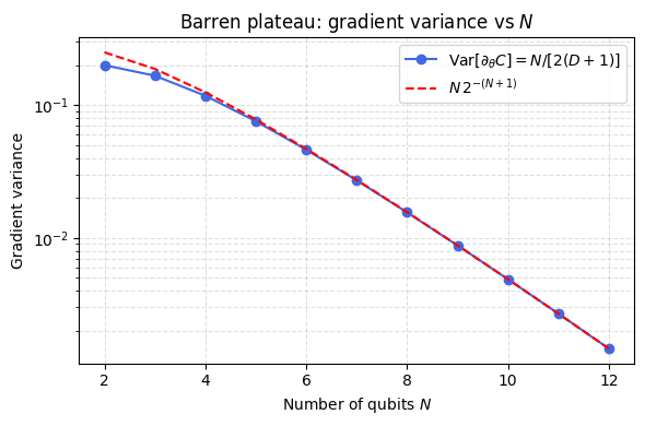
This exercise makes the connection explicit: we compute \(\mathbb{E}[C^2]\) by applying the \(k=2\) Weingarten formula term by term, showing how the permutation sums, Kronecker deltas, and trace contractions conspire to produce the exponentially small variance \(\sim N \cdot 2^{-(N+1)}\).
Preliminaries / Toolbox
Before solving this exercise, the student needs the following machinery from earlier chapters.
1. Unitary 2-design (Definition 5.1): A circuit ensemble \(\{U(\boldsymbol{\theta})\}\) is a 2-design if, for any polynomial \(P(U, U^\dagger)\) of degree \(\leq 2\) in each, \(\mathbb{E}_{\boldsymbol{\theta}}[P] = \mathbb{E}_{\mathrm{Haar}}[P]\). In practice: sufficiently deep random brickwork circuits form approximate 2-designs.
3. Tracelessness and variance: If \(\mathrm{Tr}(O) = 0\), then \(\mathbb{E}[C] = \mathrm{Tr}(O)/D = 0\) by the first moment formula, so \(\mathrm{Var}[C] = \mathbb{E}[C^2]\).
4. Parameter-shift rule: The gradient \(\partial C/\partial\theta_i\) for a Pauli rotation gate inherits the variance scaling of \(C\) up to a constant prefactor \(\sim 1/2\).
5. Pauli trace rules:\(\mathrm{Tr}(Z_j) = 0\), \(\mathrm{Tr}(Z_j^2) = D\), \(\mathrm{Tr}(Z_j Z_k) = 0\) for \(j \neq k\).
Notation:\(D = 2^N\) (Hilbert space dimension), \(|0\rangle = |0^N\rangle\) (computational zero state), \(O\) (cost observable).
Exercise
A parametrized circuit on \(N\) qubits forms a unitary 2-design. The cost function is
This is a \(k=2\) moment with indices: \(i_1 = b_1\), \(j_1 = 0\), \(i_2 = b_2\), \(j_2 = 0\), \(\ell_1 = a_1\), \(m_1 = 0\), \(\ell_2 = a_2\), \(m_2 = 0\).
Step 2: Apply the Weingarten formula
Substituting into the \(k=2\) formula, the \(j\)-deltas all become \(\delta_{0, 0_{\sigma(a)}} = 1\) for both permutations (since all \(j\)’s and \(m\)’s are 0):
%matplotlib inlineimport numpy as npimport matplotlib.pyplot as pltN_vals = np.arange(2, 13)D_vals =2.0**N_vals# Gradient variance for O = sum_j Z_j: Var[dC/dtheta] = Var[C]/2 = N / [2(D+1)]grad_var = N_vals / (2* (D_vals +1))plt.figure(figsize=(6, 4))plt.semilogy(N_vals, grad_var, 'o-', color='royalblue', label=r'$\mathrm{Var}[\partial_\theta C] = N/[2(D+1)]$')plt.semilogy(N_vals, N_vals *2.0**(-(N_vals +1)), 'r--', label=r'$N\,2^{-(N+1)}$')plt.xlabel('Number of qubits $N$')plt.ylabel('Gradient variance')plt.title('Barren plateau: gradient variance vs $N$')plt.legend()plt.grid(True, which='both', ls='--', alpha=0.4)plt.tight_layout()plt.show()
Takeaway
For a 2-design circuit and a traceless observable the cost variance is \(\mathrm{Tr}(O^2)/[D(D+1)]\), which for \(O=\sum_j Z_j\) gives \(N/(D+1)\approx N\,2^{-N}\). Gradients vanish exponentially in \(N\), so the shot budget needed to resolve one grows like \(2^N\) and rules out naive training of deep unstructured ansätze.
Connections
The gradient variance computed here is a Haar second moment, the same twirl evaluated for the Page formula and the classical shadows channel. The factor one over the dimension that sets the mean purity of a typical state is, with a different observable, the variance that flattens the training landscape, so the same typicality that makes random states useful in physics makes random circuits untrainable. The cure by observable locality is in local versus global cost, and the metrology view is in the quantum Fisher information notebook.
References
McClean et al., Barren plateaus in quantum neural network training landscapes, Nature Communications (2018).
Cerezo et al., Cost function dependent barren plateaus in shallow parametrized quantum circuits, Nature Communications (2021).
Larocca et al., Barren plateaus in variational quantum computing, Nature Reviews Physics (2025).
Holmes et al., Connecting ansatz expressibility to gradient magnitudes and barren plateaus, PRX Quantum (2022).
Płodzień, Information Scrambling, Quantum Chaos, and Haar-Random States, lecture notes (2025). arXiv:2511.14397