Overlap of Haar-Random States and Measure Concentration

Haar Measure & Weingarten Calculus, numerical solution.

Overlap of Haar-Random States and Measure Concentration

---

Background

Pick two pure states independently at random from a \(D\)-dimensional Hilbert space, each drawn uniformly in the sense of the Haar measure, and ask how aligned they are. The natural measure of alignment is the squared overlap \(\chi = |\langle\psi|\phi\rangle|^2\), which runs from zero for orthogonal states to one when the two coincide. Since the states are random, \(\chi\) is itself a random number, and the object worth studying is its distribution.

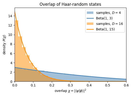
That distribution turns out to be simple, a \(\mathrm{Beta}(1, D-1)\) law with density that decays as \((1-\chi)^{D-2}\). Its mean is \(1/D\), so in a large space two independent states are typically almost orthogonal. The spread shrinks at the same \(1/D\) rate as the mean, so the overlap concentrates toward zero in absolute terms even though its relative fluctuation stays of order one. As the dimension grows the overlap piles up near zero.

This is the simplest face of concentration of measure, the phenomenon in which a smooth function of a high-dimensional random vector clusters tightly around its average. Concentration is what licenses typicality arguments, where a single random state is allowed to stand in for the ensemble because almost every state behaves the same way. The overlap distribution is a clean place to watch this happen with an exact formula in hand.

A common misreading treats the small mean as a claim about one specific pair of states rather than about the law they are drawn from. The notebook computes the mean and variance directly from the density and confirms that the typical overlap and its absolute spread both vanish as \(D\) increases.

Mathematical background

The overlap distribution follows from the geometry of the sphere alone. By unitary invariance fix \(|\psi\rangle = (1,0,\dots,0)\), so that \(\chi = |\langle\psi|\phi\rangle|^2 = |\phi_1|^2\) for a random \(|\phi\rangle\) on \(S^{2D-1}\). The squared moduli \(\{|\phi_i|^2\}\) are uniform on the simplex \(\sum_i |\phi_i|^2 = 1\), a flat Dirichlet distribution, and integrating out all but the first coordinate leaves

\[ P(\chi) = (D-1)(1-\chi)^{D-2}, \qquad 0 \le \chi \le 1, \]

the \(\mathrm{Beta}(1, D-1)\) law. Its mean is \(\mathbb{E}[\chi] = 1/D\) and its variance is \(\mathrm{Var}(\chi) = (D-1)/[D^2(D+1)]\), so the standard deviation is of order \(1/D\), the same order as the mean. The typical overlap magnitude is \(|\langle\psi|\phi\rangle| \sim D^{-1/2}\), and an atypically large overlap is exponentially suppressed,

\[ \Pr\big(|\langle\psi|\phi\rangle|^2 > \epsilon\big) \le e^{-c D \epsilon}, \]

so two random states in a large Hilbert space are almost always nearly orthogonal. The overlap concentrates toward zero in absolute terms while its relative spread stays of order one, which is why it does not self-average in the relative sense.

Exercise

The squared overlap \(\chi = |\langle\psi|\phi\rangle|^2\) between two independent Haar-random pure states in \(D\) dimensions has density:

\[ P(\chi) = (D-1)(1-\chi)^{D-2}, \qquad \chi \in [0, 1]. \]

(This is a \(\mathrm{Beta}(1, D-1)\) distribution.)

(a) Compute \(\mathbb{E}[\chi]\) and verify \(\mathbb{E}[\chi] = 1/D\).

(b) Compute \(\mathrm{Var}(\chi)\) and show it scales as \(1/D^2\) for large \(D\).

Solution

Part (a): Mean overlap

Using the substitution \(u = 1 - \chi\), we have \(\chi = 1 - u\), \(d\chi = -du\):

\[ \mathbb{E}[\chi] = (D-1)\int_0^1 \chi(1-\chi)^{D-2}\,d\chi = (D-1)\int_0^1 (1-u)\, u^{D-2}\, du. \]

Expanding:

\[ = (D-1)\left[\frac{1}{D-1} - \frac{1}{D}\right] = 1 - \frac{D-1}{D} = \frac{1}{D}. \]

\[ \boxed{\mathbb{E}[\chi] = \frac{1}{D}.} \]

Two random states have expected overlap \(1/D\), they are nearly orthogonal in high dimensions.

Part (b): Variance

First compute the second moment:

\[ \mathbb{E}[\chi^2] = (D-1)\int_0^1 (1-u)^2\, u^{D-2}\, du = (D-1)\left[\frac{1}{D-1} - \frac{2}{D} + \frac{1}{D+1}\right]. \]

Simplifying:

\[ \mathbb{E}[\chi^2] = 1 - \frac{2(D-1)}{D} + \frac{D-1}{D+1} = \frac{2}{D(D+1)}. \]

The variance is:

\[ \mathrm{Var}(\chi) = \frac{2}{D(D+1)} - \frac{1}{D^2} = \frac{2D - (D+1)}{D^2(D+1)} = \frac{D-1}{D^2(D+1)}. \]

\[ \boxed{\mathrm{Var}(\chi) = \frac{D-1}{D^2(D+1)} \sim \frac{1}{D^2} \quad \text{as } D \to \infty.} \]

The standard deviation scales as \(1/D\), the same order as the mean itself, so the relative fluctuation \(\sigma/\mu \to 1\) stays of order one. The overlap concentrates in absolute terms, with mean and spread both shrinking as \(1/D\), so two random states become orthogonal as \(D\) grows. It does not, however, self-average in the relative sense.

---

Symbolic Verification (SymPy)

Code

import sympy as sp

D = sp.Symbol('D', positive=True, integer=True)

# Haar overlap: E[|<psi|phi>|^2] = 1/D  (first moment)
E_overlap = sp.Rational(1, 1) / D
print(f'E[|<psi|phi>|^2] = {E_overlap}')

# Second moment: E[|<psi|phi>|^4] = 2/(D(D+1))
E_overlap4 = sp.Rational(2, 1) / (D * (D + 1))
print(f'E[|<psi|phi>|^4] = {E_overlap4}')

# Variance
Var = sp.simplify(E_overlap4 - E_overlap**2)
print(f'Var[|<psi|phi>|^2] = {Var}')
expected = (D - 1) / (D**2 * (D + 1))
assert sp.simplify(Var - expected) == 0
print(f'Verified: (D-1)/[D^2(D+1)]')

# For large D, overlaps ~ Exp(D): concentrated near 0
print(f'\nTypical overlap for N qubits:')
for n in range(2, 12):
    d = 2**n
    print(f'  N={n:2d}: E[overlap] = {1/d:.6f}')

E[|<psi|phi>|^2] = 1/D
E[|<psi|phi>|^4] = 2/(D*(D + 1))
Var[|<psi|phi>|^2] = (D - 1)/(D**2*(D + 1))
Verified: (D-1)/[D^2(D+1)]

Typical overlap for N qubits:
  N= 2: E[overlap] = 0.250000
  N= 3: E[overlap] = 0.125000
  N= 4: E[overlap] = 0.062500
  N= 5: E[overlap] = 0.031250
  N= 6: E[overlap] = 0.015625
  N= 7: E[overlap] = 0.007812
  N= 8: E[overlap] = 0.003906
  N= 9: E[overlap] = 0.001953
  N=10: E[overlap] = 0.000977
  N=11: E[overlap] = 0.000488

---

Numerical Verification

Code

import numpy as np
from scipy.stats import unitary_group

np.random.seed(42)

print(f"{'D':>5s}  {'E[χ]':>8s}  {'1/D':>8s}  {'Var(χ)':>10s}  {'pred':>10s}  {'σ/μ':>8s}")
print(f"{'─'*5:>5s}  {'─'*8:>8s}  {'─'*8:>8s}  {'─'*10:>10s}  {'─'*10:>10s}  {'─'*8:>8s}")

for D in [2, 4, 8, 16, 32]:
    n_samples = 20000
    overlaps = []
    for _ in range(n_samples):
        psi = unitary_group.rvs(D)[:, 0]
        phi = unitary_group.rvs(D)[:, 0]
        overlaps.append(abs(psi.conj() @ phi)**2)

    E_chi = np.mean(overlaps)
    V_chi = np.var(overlaps)
    V_pred = (D-1) / (D**2*(D+1))
    rel = np.sqrt(V_chi) / E_chi

    print(f"{D:5d}  {E_chi:8.4f}  {1/D:8.4f}  {V_chi:10.6f}  {V_pred:10.6f}  {rel:8.4f}")
    assert abs(E_chi - 1/D) < 0.01

print("\nConcentration: absolute spread σ → 0, but σ/μ → 1 (order one).")

    D      E[χ]       1/D      Var(χ)        pred       σ/μ
─────  ────────  ────────  ──────────  ──────────  ────────

    2    0.5015    0.5000    0.083250    0.083333    0.5754

    4    0.2505    0.2500    0.037646    0.037500    0.7744

    8    0.1251    0.1250    0.012067    0.012153    0.8779

   16    0.0626    0.0625    0.003420    0.003447    0.9343

   32    0.0311    0.0312    0.000925    0.000917    0.9770

Concentration: absolute spread σ → 0, but σ/μ → 1 (order one).

Code

%matplotlib inline
import matplotlib.pyplot as plt

fig, ax = plt.subplots(figsize=(6, 4))
chi_grid = np.linspace(0, 1, 400)
for D, color in zip([4, 16], ['steelblue', 'darkorange']):
    samples = np.array([abs(unitary_group.rvs(D)[:, 0].conj()
                            @ unitary_group.rvs(D)[:, 0])**2
                        for _ in range(20000)])
    ax.hist(samples, bins=50, range=(0, 1), density=True, alpha=0.5,
            color=color, label=f'samples, $D={D}$')
    ax.plot(chi_grid, (D-1)*(1-chi_grid)**(D-2), color=color, lw=2,
            label=f'Beta(1, {D-1})')
ax.set_xlim(0, 0.6)
ax.set_xlabel(r'overlap $\chi = |\langle\psi|\phi\rangle|^2$')
ax.set_ylabel(r'density $P(\chi)$')
ax.set_title('Overlap of Haar-random states')
ax.legend()
plt.show()

Takeaway

The overlap density is \((D-1)(1-\chi)^{D-2}\) with mean \(1/D\), and as \(D\) grows it piles up near zero. Two independent random states are then almost orthogonal with overwhelming probability.

Connections

The overlap of two random states is the simplest place to watch concentration of measure at work. Its mean is one over the dimension and its fluctuations shrink as the dimension grows, which is the same mechanism, in a more elaborate setting, behind the Page formula and purity concentration. The same shrinking of fluctuations is what makes quantum kernels and extreme learning machine features collapse and obstruct training.

References

• Mele, Introduction to Haar Measure Tools in Quantum Information: A Beginner’s Tutorial, Quantum (2024). doi
• Życzkowski and Sommers, Induced measures in the space of mixed quantum states, Journal of Physics A: Mathematical and General (2001).
• Nadal et al., Statistical Distribution of Quantum Entanglement for a Random Bipartite State, Journal of Statistical Physics (2011). doi
• Płodzień, Information Scrambling, Quantum Chaos, and Haar-Random States, lecture notes (2025). arXiv:2511.14397