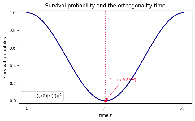
A quantum state evolving under a fixed Hamiltonian needs time to change appreciably, and there is a floor on how little time it can take to become fully distinguishable from where it started. Distinguishable here means orthogonal, so the overlap with the initial state has dropped to zero. This minimum time is controlled by a single number, the energy uncertainty \(\Delta H\) of the initial state, with a smaller spread in energy forcing slower change.
The precise statement is the Mandelstam-Tamm bound, which sets the time to reach orthogonality at \(T_\perp = \pi/(2\Delta H)\). A state with sharply defined energy barely moves, while a state spread over a wide band of energies can turn over quickly. The bound holds for any Hamiltonian and any initial state, so it places a universal limit on the speed of unitary dynamics.
There is a geometric way to read the same result. The evolution \(U(t) = e^{-iHt}\) traces a path on the unitary group, and with the metric inherited from the Hilbert-Schmidt inner product this path is a geodesic traversed at constant speed. The state moves along the shortest route available to it, and the energy uncertainty plays the role of how fast it covers ground. A qubit prepared in an eigenstate of \(\sigma_z\) and driven by \(H = (\omega/2)\sigma_x\) has the largest spread its energy range allows. Its survival probability is \(\cos^2(\omega t/2)\), which first reaches zero exactly at \(T_\perp\), so the qubit saturates the bound.
The notebook computes the geodesic length and the orthogonality time and confirms that this qubit sits right at the limit.
Mathematical background
The geometric reading rests on the length of a path on \(U(D)\). With the Hilbert-Schmidt metric \(\langle X, Y\rangle = -\mathrm{Tr}(XY)\) on the skew-Hermitian algebra, the length of a curve \(U(t)\) is
\[
L[U(t)] = \int_0^1 \sqrt{\langle \dot U U^\dagger, \dot U U^\dagger\rangle}\,dt = \int_0^1 \sqrt{\mathrm{Tr}(\dot U^\dagger \dot U)}\,dt ,
\]
where the second form follows because \(\dot U U^\dagger\) is skew-Hermitian and the trace is cyclic. For evolution under a fixed Hamiltonian, \(U(t) = e^{-iHt}\) gives \(\dot U = -iHU\) and \(\mathrm{Tr}(\dot U^\dagger \dot U) = \mathrm{Tr}(H^2)\), a constant. The path is therefore a geodesic traversed at constant speed \(\sqrt{\mathrm{Tr}(H^2)}\), and its length grows linearly in time. Restricted to the evolving state, the speed in the Fubini-Study metric is set by the energy uncertainty \(\Delta H = \sqrt{\langle H^2\rangle - \langle H\rangle^2}\), which is what turns the geometric length into the Mandelstam-Tamm time \(T_\perp = \pi/(2\Delta H)\) to reach an orthogonal state.
Motivation
How fast can a quantum state evolve? The quantum speed limit (Mandelstam-Tamm bound) sets a fundamental lower bound on the time needed to evolve between orthogonal states. This exercise derives the bound from the geometry of the unitary group: Hamiltonian evolution traces a geodesic on \(U(D)\) whose speed is set by the energy spread \(\Delta H\). The connection between Riemannian geometry and quantum dynamics is one of the deepest structural insights in quantum information.
Exercise
In the bi-invariant HS metric on \(U(D)\), the geodesic \(U(t) = \exp(-iHt)\) has constant speed \(\|dU/dt \cdot U^\dagger\| = \sqrt{\mathrm{Tr}(H^2)}\).
(a) Compute the geodesic length from \(I\) to \(U(T) = \exp(-iHT)\).
(b) For \(H = (\omega/2)\sigma_x\) on a qubit, compute the speed and the length to \(U(\pi/\omega) = -i\sigma_x\).
(c) Mandelstam-Tamm bound: for \(|\psi_0\rangle = |0\rangle\), compute \(\Delta H\), predict \(T_\perp\), and verify the survival probability vanishes at \(t = T_\perp\).
Hamiltonian evolution is a constant-speed geodesic on \(U(D)\), with speed \(\sqrt{\mathrm{Tr}(H^2)}\). For \(|0\rangle\) under \(H=(\omega/2)\sigma_x\) the survival probability is \(\cos^2(\omega t/2)\), which first vanishes exactly at \(T_\perp=\pi/\omega\), saturating the Mandelstam-Tamm bound.
Code
import numpy as npfrom scipy.linalg import expmomega =2.0sx = np.array([[0,1],[1,0]], dtype=complex)H = omega/2* sxpsi0 = np.array([1, 0], dtype=complex)T_perp = np.pi / omegadelta_H = omega /2print(f"ω = {omega}, ΔH = {delta_H}, T_⊥ = π/ω = {T_perp:.4f}")print(f"Speed = ω/√2 = {omega/np.sqrt(2):.4f}")print(f"Length at T_⊥ = π/√2 = {np.pi/np.sqrt(2):.4f}")print()times = np.linspace(0, 2*T_perp, 9)print(f"{'t/T⊥':>8s}{'|⟨0|ψ(t)⟩|²':>14s}")print(f"{'─'*8:>8s}{'─'*14:>14s}")for t_val in times: U = expm(-1j* H * t_val) p =abs(psi0.conj() @ U @ psi0)**2print(f"{t_val/T_perp:8.3f}{p:14.6f}")# Check orthogonality at T_perpU_perp = expm(-1j* H * T_perp)surv =abs(psi0.conj() @ U_perp @ psi0)**2assert surv <1e-10, f"Survival = {surv}"print(f"\nSurvival at T_⊥ = {surv:.2e}: bound saturated.")